1. Limits and Continuity#
1.1. Limit(极限) and Continuity(连续性)#
1.2. Learning Objectives#
After reading this chapter, you should be able to:
Explain what a
limitmeans intuitively and formally.Distinguish the value of a function from the limit of a function.
Determine the
domain(定义域)of common functions.Evaluate limits using direct substitution, factorization, rationalization, highest-order terms, and standard limits.
Use
equivalent infinitesimals(等价无穷小)to simplify limit problems.Determine whether a function is
continuous(连续)at a point.Identify different types of
discontinuities(间断点).Use the
Intermediate Value Theorem(介值定理)to prove that an equation has a solution.Use Python to visualize limits, continuity, and discontinuity.
1.3. Why This Topic Matters#
Calculus begins with one central question:
What happens to a function as the input gets closer and closer to a certain value?
This question is not always the same as asking what the function value is at that point.
For example, consider:
At \(x=1\), the function is not defined because the denominator becomes zero. But if we simplify:
for \(x \ne 1\). As \(x\) approaches \(1\), the function approaches:
So the function has no value at \(x=1\), but it still has a limit there.
This distinction is fundamental. Without limits, we cannot properly define derivative(导数), differential(微分), Taylor Expansion(泰勒展开), or continuity(连续性). In fact, the derivative definition in your later differential chapter is built directly from a limit of difference quotients.
Limits help us answer questions such as:
What happens near a point where a formula breaks?
Does a function approach a stable value?
Does a graph have a jump, a hole, or a vertical asymptote?
Can we approximate one function by another near a point?
Is a piecewise function continuous?
Does an equation have at least one solution in an interval?
The main idea is simple but powerful:
A limit describes where a function is going, not necessarily where it is.
1.4. Big Picture Intuition#
Imagine walking toward a house.
You may never actually enter the house, but you can still say where you are approaching. A limit works the same way.
When we write:
we mean:
As \(x\) gets closer and closer to \(a\), the function value \(f(x)\) gets closer and closer to \(L\).
The important point is that \(x\) approaches \(a\), but does not have to equal \(a\).
So the limit cares about nearby behavior, not only the value exactly at the point.
x approaches a from the left x approaches a from the right
→ → → a ← ← ←
If f(x) approaches the same value L from both sides, then the two-sided limit exists.
A function may have:
a function value but no limit,
a limit but no function value,
both a function value and a limit, but they are not equal,
both a function value and a limit that are equal.
Only the fourth case gives continuity.
1.5. Domain and Function Equivalence#
Before solving limits, we must understand where a function is defined.
1.5.1. Domain(定义域)#
The domain of a function is the set of input values for which the function is valid.
Common rules:
Expression type |
Domain restriction |
|---|---|
\(\frac{1}{g(x)}\) |
denominator cannot be \(0\) |
\(\sqrt{g(x)}\) |
\(g(x)\geq0\) |
\(\frac{1}{\sqrt{g(x)}}\) |
\(g(x)>0\) |
\(\ln(g(x))\) |
\(g(x)>0\) |
\(\arcsin x,\arccos x\) |
\(-1\leq x\leq1\) |
Example:
The denominator cannot be zero, and the square root must be real and positive:
So:
Therefore, the domain is:
1.5.2. Function Equivalence(函数相等)#
Two functions are equal only if they have:
the same domain,
the same output for every input in that domain.
For example:
is not exactly the same function as:
because \(f(x)\) is undefined at \(x=0\), while \(g(x)\) is defined at \(x=0\).
However, for limit purposes near \(x=0\), we may sometimes simplify expressions after remembering that the original function may have a missing point.
This is why domain matters.
1.6. The equivalent of functions#
The same domain and the same mapping
i. \(f(x) = \ln(x - 1) \neq g(x) = \ln\sqrt{(x - 1)^2}\)
ii. \(f(x) = \frac{x}{x} \neq g(x) = 1\)
iii. \(f(x) = \sqrt{x^2} = g(x) = |x|\)
iv. \(f(x) = \begin{cases} -x, & x \geq 1 \\ 1, & x < 1 \end{cases} \neq g(x) = \begin{cases} 0, & x = 1 \\ 1, & x < 1 \end{cases}\)
1.7. Formal Definition of a Limit#
The formal definition is the \(\epsilon\)-\(\delta\) definition(\(\epsilon\)-\(\delta\)定义).
We say:
if for every:
there exists:
such that:
whenever:
1.8. What the symbols mean#
\(a\): the input value that \(x\) approaches
\(L\): the value that \(f(x)\) approaches
\(\epsilon\): how close we want \(f(x)\) to be to \(L\)
\(\delta\): how close \(x\) must be to \(a\)
\(0<|x-a|\): \(x\) is near \(a\), but not equal to \(a\)
In words:
No matter how small a target distance \(\epsilon\) we choose around \(L\), we can find a small enough input distance \(\delta\) around \(a\), so that all nearby \(x\)-values make \(f(x)\) fall inside the target distance.
This is a precise way to express “getting close.”
1.8.1. Figure Demo 1: Visualizing the \(\epsilon\)-\(\delta\) Idea#
1.9. The definition of limit#
Let \(f(x)\) be a function defined on an interval that contains \(x = a\), except possibly at \(x = a\). Then we say that,
if for every number \(\epsilon > 0\) there is some number \(\delta > 0\) such that
import numpy as np
import matplotlib.pyplot as plt

plt.rcParams.update({
    "font.size": 11,
    "axes.titlesize": 13,
    "axes.labelsize": 11,
    "legend.fontsize": 10,
    "figure.dpi": 120
})

def f(x):
    return 2*x + 1

a = 2
L = f(a)

epsilon = 0.6
delta = epsilon / 2

x = np.linspace(0.5, 3.5, 400)
y = f(x)

plt.figure(figsize=(8, 5))
plt.plot(x, y, label=r"$f(x)=2x+1$")
plt.axvline(a, linestyle="--", label=r"$x=a$")
plt.axhline(L, linestyle="--", label=r"$L=f(a)$")

plt.axhspan(L - epsilon, L + epsilon, alpha=0.15, label=r"$L\pm\epsilon$")
plt.axvspan(a - delta, a + delta, alpha=0.15, label=r"$a\pm\delta$")

plt.xlabel("x")
plt.ylabel("f(x)")
plt.title(r"Visualizing the $\epsilon$-$\delta$ Definition")
plt.legend()
plt.grid(True, alpha=0.3)
plt.show()
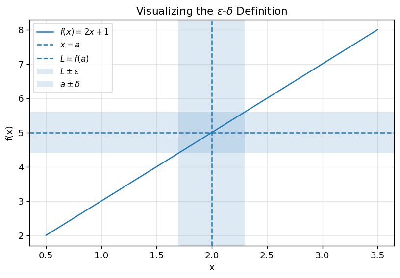
What this figure teaches:
If \(x\) is kept within the \(\delta\)-window around \(a\), then \(f(x)\) stays within the \(\epsilon\)-window around \(L\).
1.10. How to Solve Limit Problems Step by Step#
A useful workflow is:
Step 1: Check the domain.
Step 2: Try direct substitution.
Step 3: If direct substitution works, stop.
Step 4: If it gives 0/0 or another indeterminate form, simplify.
Step 5: Use factorization, rationalization, standard limits, equivalent infinitesimals, or L’Hôpital’s Rule.
Step 6: Interpret the result.
1.11. Solve the limit Problem#
1.12. Substitute Directly#
1.12.1. L’Hopital’s Law#
i. Infinity to infinity
ii. Infinity small to infinity small
Try the simplest valid method first.
1.13. Core Techniques for Solving Limits#
1.14. Direct Substitution#
If \(f(x)\) is continuous at \(x=a\), then:
Example:
Direct substitution is the first method you should try.
1.14.1. Factorization#
Example:
Direct substitution gives:
Factor the denominator:
So:
for \(x\neq1\).
Therefore:
This is not saying the original expression is defined at \(x=1\). It says the nearby behavior is equivalent for the purpose of the limit.
1.14.2. Rationalization(有理化)#
Example:
Direct substitution gives:
Multiply numerator and denominator by the conjugate:
Then:
The denominator becomes:
So:
for \(x\neq4\).
Therefore:
1.14.3. Highest-Order Terms for \(x\to\infty\)#
For rational functions, the highest power of \(x\) usually controls the limit.
Example 1:
The numerator and denominator have the same highest degree, so the limit is the ratio of leading coefficients.
Example 2:
The denominator grows faster.
Example 3:
The numerator grows faster.
1.14.4. Figure Demo 2: Highest-Order Terms Dominate#
1.15. The Property of infinity (∞) and infinity small (0)#
The product of infinity small with bounded function (e.g., \(\sin x \), \(\cos x \), \(\arctan x \), \(arccot x \)) is infinity small.
- \[ \lim_{x \to \infty} \frac{\sin x}{x} = \lim_{x \to \infty} \sin x \ast \frac{1}{x} = 0 \]
- \[ \lim_{x \to 2} (x - 2) \sin \frac{1}{x - 2} = \lim_{u \to \infty} \frac{\sin u}{u} = 0 \]
1.16. Three special cases#
Factorization
Rationalization of numerator and denominator
Get the highest order \(x\to \infty\)
import numpy as np
import matplotlib.pyplot as plt

x = np.linspace(1, 100, 500)

f1 = (2*x**3 + 3*x**2 + 5) / (7*x**3 + 4*x**2 - 1)
f2 = (3*x**2 + 5) / (7*x**3 + 4*x**2 - 1)

plt.figure(figsize=(8, 5))
plt.plot(x, f1, label=r"$\frac{2x^3+3x^2+5}{7x^3+4x^2-1}$")
plt.plot(x, f2, label=r"$\frac{3x^2+5}{7x^3+4x^2-1}$")
plt.axhline(2/7, linestyle="--", label=r"$2/7$")
plt.axhline(0, linestyle=":", label="0")

plt.xlabel("x")
plt.ylabel("function value")
plt.title("Highest-Order Terms Control Limits at Infinity")
plt.legend()
plt.grid(True, alpha=0.3)
plt.show()
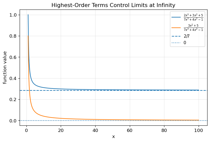
What this figure teaches:
As \(x\) becomes large, lower-order terms become relatively less important. The leading terms determine the long-run behavior.
1.17. Important Limit Results#
1.18. The Sine Limit#
One of the most important limits is:
This means:
as \(x\to0\).
In words:
Near zero, \(\sin x\) behaves like \(x\).
This result is foundational for later derivative and Taylor Expansion chapters. In the differential chapter, the local approximation idea \(dy=f'(x)dx\) is used to approximate small changes. In the Taylor chapter, the expansion
explains why \(\sin x\sim x\) near zero.
1.18.1. Figure Demo 3: Why \(\sin x\sim x\) Near Zero#
import numpy as np
import matplotlib.pyplot as plt

x = np.linspace(-1, 1, 400)

plt.figure(figsize=(8, 5))
plt.plot(x, np.sin(x), label=r"$\sin x$")
plt.plot(x, x, "--", label=r"$x$")

plt.xlabel("x")
plt.ylabel("value")
plt.title(r"Near Zero, $\sin x$ Behaves Like $x$")
plt.legend()
plt.grid(True, alpha=0.3)
plt.show()
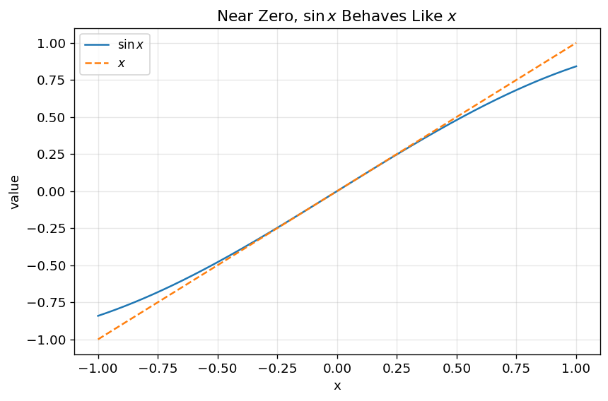
What this figure teaches:
Near \(x=0\), the curves \(y=\sin x\) and \(y=x\) almost overlap. That is the visual meaning of \(\sin x\sim x\).
1.19. The Exponential Limit#
Another fundamental limit is:
More generally:
and:
Examples:
This limit is important because it connects repeated small multiplicative changes to exponential growth.
1.20. Two important limits#
i. \(\lim_{u(x) \to 0} \frac{\sin u(x)}{u(x)} = 1\)
Prove using the definition of differential
a) \(\lim_{x \to 0} \sin x = x\)
\[ f'(x) = \frac{f(x + \delta) - f(x)}{\delta} \to f(x + \delta) = f(x) + f'(x) \ast \delta, \text{ when } \delta \to 0 \]\(\sin (x + \delta) \approx \sin x + \cos x \ast \delta\) when \(\delta \to 0\)
\(\sin \delta \approx 0 + \delta\), when \(\delta \to 0\)
Replace \(\delta\) with \(x\), \(\lim_{x \to 0} \sin x = x\)
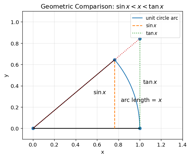
ii. \(\lim_{A \to \infty} \left(1 + \frac{1}{A}\right)^A = e\)
Prove using Taylor’s Formula
\[ e < \left(1 + \frac{1}{k}\right)^k = 1 + \frac{k}{1} \left(\frac{1}{k}\right)^1 + \frac{k(k - 1)}{1 \cdot 2} \left(\frac{1}{k}\right)^2 + \frac{k(k - 1)(k - 2)}{1 \cdot 2 \cdot 3} \left(\frac{1}{k}\right)^3 + \cdots \]a)
\[ e = 1 + \frac{1}{2!} + \frac{1}{3!} + \cdots = e \]\(\lim_{x \to \infty} \left(1 - \frac{2}{x}\right)^x = e^{-2} = \frac{1}{e^2}\)
\(\lim_{x \to 0} (1 - 2x)^{\frac{1}{x}} = e^{-2}\)
\(\lim_{x \to \infty} \left(1 + \frac{1}{n}\right)^{n+3} = e\)
import numpy as np
import matplotlib.pyplot as plt

plt.rcParams.update({
    "font.size": 11,
    "axes.titlesize": 13,
    "axes.labelsize": 11,
    "legend.fontsize": 10,
    "figure.dpi": 120
})

theta = 0.7

# Unit circle arc
arc = np.linspace(0, theta, 200)
circle_x = np.cos(arc)
circle_y = np.sin(arc)

# Key points
O = np.array([0, 0])
A = np.array([1, 0])
B = np.array([np.cos(theta), np.sin(theta)])
T = np.array([1, np.tan(theta)])

plt.figure(figsize=(6, 6))

# Unit circle arc
plt.plot(circle_x, circle_y, label="unit circle arc")

# Radius lines
plt.plot([0, A[0]], [0, A[1]], color="black")
plt.plot([0, B[0]], [0, B[1]], color="black")

# Inner triangle height sin(theta)
plt.plot([B[0], B[0]], [0, B[1]], "--", label=r"$\sin x$")

# Tangent line and outer triangle
plt.plot([1, 1], [0, T[1]], ":", label=r"$\tan x$")
plt.plot([0, T[0]], [0, T[1]], ":")

# Arc annotation
plt.text(0.82, 0.25, r"arc length = $x$", fontsize=12)
plt.text(B[0] - 0.2, B[1] / 2, r"$\sin x$", fontsize=12)
plt.text(1.03, T[1] / 2, r"$\tan x$", fontsize=12)

plt.scatter([O[0], A[0], B[0], T[0]], [O[1], A[1], B[1], T[1]])

plt.xlim(-0.1, 1.4)
plt.ylim(-0.1, 1.1)
plt.gca().set_aspect("equal", adjustable="box")
plt.xlabel("x")
plt.ylabel("y")
plt.title(r"Geometric Comparison: $\sin x < x < \tan x$")
plt.legend()
plt.grid(True, alpha=0.3)
plt.show()
1.21. Equivalent Infinitesimals#
An infinitesimal(无穷小)is a quantity that approaches \(0\).
Two infinitesimals \(f(x)\) and \(g(x)\) are equivalent if:
We write:
as \(x\to a\).
This means:
Near the limit point, \(f(x)\) and \(g(x)\) have the same leading-order behavior.
Common equivalent infinitesimals as \(x\to0\):
Important correction:
is a first-order approximation, but as an infinitesimal equivalence, the more useful form is:
because both sides approach \(0\).
1.22. Worked Example: Equivalent Infinitesimals#
Evaluate:
Use:
and:
Therefore:
If the numerator were \(\ln(1+2x)\), then:
and the result would be:
This distinction is important: the coefficient inside the small quantity matters.
1.23. Equivalence of infinity small#
i. \(\lim_{x \to 0} \frac{\sin x}{x} = 1 \to \sin x \sim x \ (\text{when } x \to 0)\)
ii. \(1 - \cos x \sim \frac{1}{2} x^2\)
Prove: \(\lim_{x \to 0} \frac{1 - \cos x}{\frac{1}{2}x^2} = \frac{\sin x}{x} = 1\)
iii. \(\ln(1 + x) \sim x\)
Prove: \(\ln(1 + x + \delta) = \ln(1 + x) + \frac{\delta}{1 + x} = \ln 1 + \delta \to \ln(1 + \delta) \approx \delta \text{ when } \delta \to 0 \text{ and } x = 0\)
\(\lim_{x \to 0} \frac{\ln(1 + x)}{\sin 3x} = \frac{2x}{3x} = \frac{2}{3}\)
iv. \(e^x - 1 \sim x\)
v. \((1 + x)^\alpha = 1 + \alpha x\)
Prove: \((1 + x + \delta)^\alpha = (1 + x)^\alpha + (\alpha \delta)(1 + x)^{\alpha - 1} \to (1 + \delta)^\alpha = 1 + \alpha \delta \text{ when } \delta \to 0 \text{ and } x = 0\)
1.24. Continuity#
A function \(f(x)\) is continuous at \(x=x_0\) if three conditions hold:
\(f(x_0)\) is defined.
\(\lim_{x\to x_0}f(x)\) exists.
\(\lim_{x\to x_0}f(x)=f(x_0)\).
In one formula:
Continuity means:
The function value agrees with the value the function approaches.
Graphically, a continuous function can be drawn near the point without lifting the pen.
1.25. Figure Demo 4: Continuous Function vs Hole vs Jump#
1.26. Continuous#
1.27. Continuous in functions#
\(f(x)\) has a definition at \(x_0\)
\(\lim_{x \to x_0} f(x) = f(x_0)\)
1.28. Example#
\(f(x) = \begin{cases} x^2 + 2a, & x \leq 0, \\ \frac{\sin x}{2x}, & x > 0 \end{cases}\)
is continuous at \(x = 0\), what’s the value of \(a\)?
Answer
\(\lim_{x \to 0} (x^2 + 2a) = 2a\), \(\lim_{x \to 0} \frac{\sin x}{2x} = \frac{1}{2} = 2a \to a = \frac{1}{4}\)
import numpy as np
import matplotlib.pyplot as plt

x_left = np.linspace(-2, 0, 200, endpoint=False)
x_right = np.linspace(0, 2, 200)

x = np.linspace(-2, 2, 400)

continuous = x**2
hole = (x**2 - 1) / (x - 1)
jump_left = x_left + 1
jump_right = x_right + 2

fig, axes = plt.subplots(1, 3, figsize=(12, 3.8))

axes[0].plot(x, continuous)
axes[0].set_title("Continuous")
axes[0].set_xlabel("x")
axes[0].set_ylabel("f(x)")
axes[0].grid(True, alpha=0.3)

x_hole = np.linspace(-2, 2, 400)
x_hole = x_hole[np.abs(x_hole - 1) > 0.02]
axes[1].plot(x_hole, (x_hole**2 - 1)/(x_hole - 1))
axes[1].scatter([1], [2], facecolors="white", edgecolors="black", s=80)
axes[1].set_title("Removable Discontinuity")
axes[1].set_xlabel("x")
axes[1].grid(True, alpha=0.3)

axes[2].plot(x_left, jump_left)
axes[2].plot(x_right, jump_right)
axes[2].scatter([0], [1], facecolors="white", edgecolors="black", s=80)
axes[2].scatter([0], [2], s=80)
axes[2].set_title("Jump Discontinuity")
axes[2].set_xlabel("x")
axes[2].grid(True, alpha=0.3)

plt.tight_layout()
plt.show()
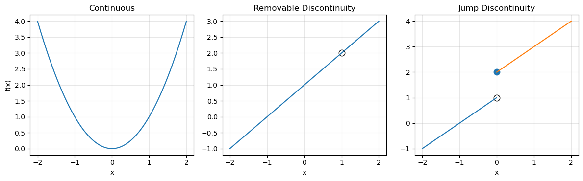
What this figure teaches:
A continuous function has no break. A removable discontinuity has a hole. A jump discontinuity has different left-hand and right-hand limits.
1.29. Worked Example: Piecewise Continuity#
Suppose:
Find \(a\) so that \(f(x)\) is continuous at \(x=0\).
1.30. Step 1: Compute the left-hand value#
For \(x\leq0\):
So:
1.30.1. Step 2: Compute the right-hand limit#
For \(x>0\):
Using:
we get:
1.30.2. Step 3: Set left and right behavior equal#
For continuity:
Therefore:
So the function is continuous at \(x=0\) when:
1.31. Discontinuities and Break Points#
A discontinuity(间断点)occurs when a function is not continuous at a point.
Common types:
1.31.1. Undefined Point#
Example:
At:
the denominator is \(0\), so the function is undefined.
As \(x\to3\), the function grows without bound. This is an infinite discontinuity(无穷间断点).
1.31.2. Limit Does Not Exist#
Example:
The left-hand limit and right-hand limit are different at \(x=0\). So the two-sided limit does not exist.
1.31.3. Limit Exists but Does Not Equal the Function Value#
Example:
Then:
but:
So the function is not continuous at \(x=1\), even though the limit exists.
1.32. The break points of functions#
The point with invalid definition
The point with no limits
a. \(x = 3\) for \(f(x) = \frac{x^2 + 1}{x - 3}\), with limit \(= \infty\)
The point with limit that does not equal to its function value
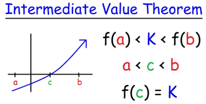
1.33. Intermediate Value Theorem#
The Intermediate Value Theorem(介值定理)says:
If \(f(x)\) is continuous on the closed interval:
and \(k\) is any number between:
and:
then there exists at least one point:
such that:
In simpler words:
A continuous function cannot jump over a value.
If the graph moves continuously from below zero to above zero, it must cross zero somewhere.
1.34. Worked Example: Proving an Equation Has a Solution#
Prove that:
has a solution in:
Let:
Evaluate at the endpoints:
So:
and:
Since \(f(x)\) is a polynomial, it is continuous on \([0,1]\).
Because \(0\) lies between \(f(0)=1\) and \(f(1)=-2\), the Intermediate Value Theorem guarantees that there exists some:
such that:
Therefore, the equation has at least one solution in \((0,1)\).
1.34.1. Figure Demo 5: Intermediate Value Theorem#
1.35. The Intermediate Value Theorem#
If \(f(x)\) is continuous on the closed interval \([a, b]\) and \(k\) is any number between \(f(a)\) and \(f(b)\), then there exists at least one value \(c\) in the interval \((a, b)\) such that \(f(c) = k\).
a. Prove there is a solution of \(x^3 - 4x^2 + 1 = 0\) on the interval \((0,1)\).
import numpy as np
import matplotlib.pyplot as plt

def f(x):
    return x**3 - 4*x**2 + 1

x = np.linspace(0, 1, 400)
y = f(x)

plt.figure(figsize=(8, 5))
plt.plot(x, y, label=r"$f(x)=x^3-4x^2+1$")
plt.axhline(0, linestyle="--", label="y = 0")
plt.scatter([0, 1], [f(0), f(1)], zorder=5, label="Endpoint values")

plt.xlabel("x")
plt.ylabel("f(x)")
plt.title("Intermediate Value Theorem: A Root Must Exist")
plt.legend()
plt.grid(True, alpha=0.3)
plt.show()
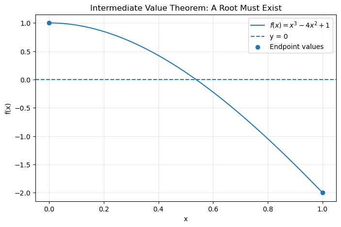
What this figure teaches:
The continuous curve starts above zero and ends below zero. Therefore, it must cross the \(x\)-axis at least once.
1.36. Python Lab: Numerically Exploring Limits and Continuity#
In this lab, we will visualize three ideas:
a removable discontinuity,
a one-sided jump,
a limit at infinity.
1.37. Lab 1: Removable Discontinuity#
import numpy as np
import matplotlib.pyplot as plt

def f_original(x):
    return (x**2 - 1) / (x - 1)

def f_simplified(x):
    return x + 1

x = np.linspace(-2, 4, 500)
x_plot = x[np.abs(x - 1) > 0.03]

plt.figure(figsize=(8, 5))
plt.plot(x_plot, f_original(x_plot), label=r"$\frac{x^2-1}{x-1}$")
plt.plot(x, f_simplified(x), "--", label=r"$x+1$")

plt.scatter([1], [2], facecolors="white", edgecolors="black", s=90, label="missing point")

plt.xlabel("x")
plt.ylabel("f(x)")
plt.title("A Limit Can Exist Even When the Function Is Undefined")
plt.legend()
plt.grid(True, alpha=0.3)
plt.show()
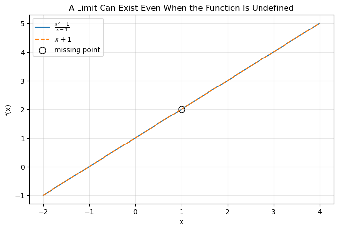
Interpretation:
The original function is undefined at \(x = 1\), but its nearby behavior approaches \(2\).
1.38. Lab 2: One-Sided Limits#
import numpy as np
import matplotlib.pyplot as plt

x_left = np.linspace(-2, 0, 200, endpoint=False)
x_right = np.linspace(0, 2, 200)

y_left = np.ones_like(x_left)
y_right = 2 * np.ones_like(x_right)

plt.figure(figsize=(8, 5))
plt.plot(x_left, y_left, label="left branch")
plt.plot(x_right, y_right, label="right branch")
plt.scatter([0], [1], facecolors="white", edgecolors="black", s=90)
plt.scatter([0], [2], s=90)

plt.xlabel("x")
plt.ylabel("f(x)")
plt.title("Two-Sided Limit Does Not Exist When One-Sided Limits Differ")
plt.legend()
plt.grid(True, alpha=0.3)
plt.show()
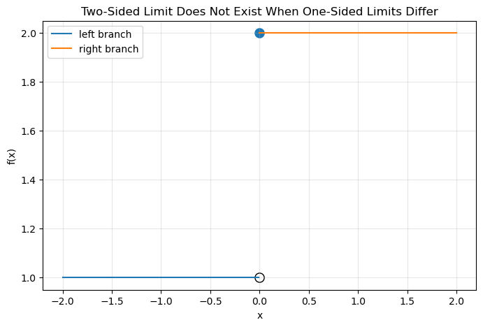
Interpretation:
As \(x \to 0^-\), the function approaches \(1\).
As \(x \to 0^+\), the function approaches \(2\).
Since the two one-sided limits are different, the two-sided limit does not exist.
1.39. Lab 3: Limit at Infinity#
import numpy as np
import matplotlib.pyplot as plt

x = np.linspace(1, 200, 800)

y = (2*x**3 + 3*x**2 + 5) / (7*x**3 + 4*x**2 - 1)

plt.figure(figsize=(8, 5))
plt.plot(x, y, label="rational function")
plt.axhline(2/7, linestyle="--", label=r"limit = $2/7$")

plt.xlabel("x")
plt.ylabel("function value")
plt.title("A Rational Function Approaches the Ratio of Leading Coefficients")
plt.legend()
plt.grid(True, alpha=0.3)
plt.show()
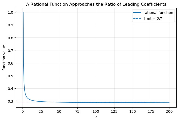
Interpretation:
As \(x\) grows, the function approaches:
because the cubic terms dominate.
1.40. How to Interpret the Results#
1.41. A Limit Is About Nearby Behavior#
When evaluating:
we are asking what happens near \(a\), not necessarily at \(a\).
This is why a function can have a limit at a point where it is not defined.
1.41.1. A Function Value Is Not the Same as a Limit#
The value \(f(a)\) is the function’s output at \(a\).
The limit \(\lim_{x\to a}f(x)\) is the value the function approaches near \(a\).
They may be different.
1.41.2. Continuity Requires Agreement#
A function is continuous at \(a\) only when:
If the limit exists but does not equal the function value, the function is not continuous.
1.41.3. Equivalent Infinitesimals Are Local Replacements#
When we write:
as \(x\to0\), it does not mean \(\sin x=x\) everywhere.
It means their ratio approaches 1 near zero.
1.42. Common Pitfalls and Misunderstandings#
1.42.1. Pitfall 1: Substituting Directly When the Function Is Not Continuous#
Direct substitution works only when the function is continuous at the target point.
If substitution gives:
you need more work.
1.42.2. Pitfall 2: Treating \(0/0\) as 0#
The expression:
is not equal to 0. It is an indeterminate form(未定式).
For example:
but:
The same symbolic form can lead to different limits.
1.42.3. Pitfall 3: Forgetting Domain Changes After Simplification#
can be simplified to 1 only for:
As functions, they are not identical because their domains are different.
1.42.4. Pitfall 4: Misusing Equivalent Infinitesimals#
Equivalent infinitesimals are valid only under a specific limiting process.
For example:
as \(x\to0\), not as \(x\to\infty\).
1.42.5. Pitfall 5: Forgetting One-Sided Limits#
A two-sided limit exists only if both one-sided limits exist and are equal:
If they differ, the two-sided limit does not exist.
1.44. Summary#
A limit describes the value a function approaches as the input approaches a point.
The core notation is:
The central intuition is:
A limit is about where the function is going, not necessarily where it is.
Continuity adds one more requirement:
Limits are the foundation for derivative, differential, L’Hôpital’s Rule, Taylor Expansion, and much of calculus.
One memorable sentence:
Limits teach us how to understand a function by looking near a point, even when the point itself is problematic.
1.45. Quiz#
1.45.1. Conceptual Questions#
1.45.1.1. Q1: What does \(\lim_{x\to a}f(x)=L\) mean?#
A. \(f(a)=L\) must be true
B. \(f(x)\) approaches \(L\) as \(x\) approaches \(a\)
C. \(x\) must equal \(a\)
D. \(f(x)\) is always equal to \(L\)
Answer
Correct answer: B.
A limit describes nearby behavior as \(x\) approaches \(a\). It does not necessarily require \(f(a)=L\).
1.45.1.2. Q2: When is a function continuous at \(x=a\)?#
A. \(f(a)\) is undefined
B. \(\lim_{x\to a}f(x)\) exists but differs from \(f(a)\)
C. \(\lim_{x\to a}f(x)=f(a)\)
D. The left-hand limit and right-hand limit are always different
Answer
Correct answer: C.
Continuity requires the function value and the limit to exist and be equal.
1.45.1.3. Q3: Why are \(f(x)=x/x\) and \(g(x)=1\) not exactly the same function?#
A. They always produce different outputs
B. \(x/x\) is undefined at \(x=0\), while 1 is defined at \(x=0\)
C. 1 is not a function
D. \(x=0\)
Answer
Correct answer: B.
The two expressions agree for \(x\neq0\), but they have different domains.
1.45.1.4. Q4: What does \(\sin x\sim x\) as \(x\to0\) mean?#
A. \(\sin x=x\) for every \(x\)
B. \(\sin x\) and \(x\) have the same value everywhere
C.
as \(x\to0\)
D. \(\sin x/x\to0\) as \(x\to0\)
Answer
Correct answer: C.
Equivalent infinitesimals have a ratio that approaches 1 near the limiting point.
1.45.1.5. Q5: What does the Intermediate Value Theorem require?#
A. The function must be continuous on a closed interval
B. The function must be differentiable everywhere
C. The function must be linear
D. The function must have no roots
Answer
Correct answer: A.
The theorem requires continuity on \([a,b]\). Then the function must take every value between \(f(a)\) and \(f(b)\).
1.45.2. Applied Questions#
1.45.2.1. Q6: Evaluate#
A. 0
B. 1
C. \(\frac{1}{2}\)
D. Does not exist
Answer
Correct answer: C.
Factor the denominator:
Then:
for \(x\neq1\). Therefore:
1.45.2.2. Q7: Find \(a\) so that the function is continuous at \(x=0\):#
A. \(\frac{1}{2}\)
B. \(\frac{1}{4}\)
C. 1
D. 0
Answer
Correct answer: B.
Left-hand value:
Right-hand limit:
Set them equal:
So:
1.45.3. Explain in Your Own Words#
1.45.3.1. Q8: Explain the difference between a function value, a limit, and continuity.#
Answer
A function value \(f(a)\) is the output exactly at \(x=a\). A limit \(\lim_{x\to a}f(x)\) is the value the function approaches as \(x\) gets close to \(a\). Continuity means these two agree: the function is defined at \(a\), the limit exists, and the limit equals the function value.