10. Spatial Autocorrelation#
10.1. Spatial Randomness#
10.1.1. The Null Hypothesis#
Spatial randomness is absence of any pattern
If rejected, then there is evidence of spatial structure
10.1.2. Interpreting Spatial Randomness#
The observed spatial pattern of clues is equally likely as any other spatial pattern
Simultaneousview (Pattern)
Value at one location does not depend on values at other (neighboring) locations
Conditionalview
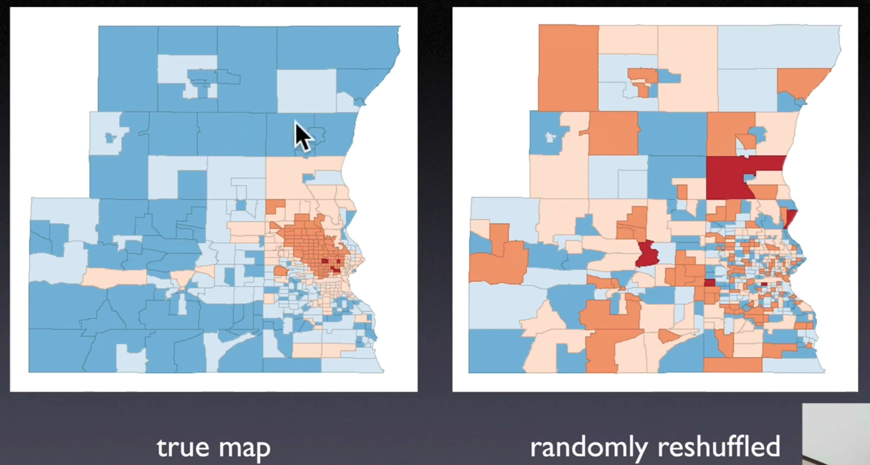
10.1.3. Operationalizing Spatial Randomness#
Random permutation or reshuffling of values
Tobler's First Law of Geography
Everything depends on everything else, but closer things more so
Structures spatial dependence
Importance of
distance decayObservations further apart are less correlate
Range of interaction- no spatial correlation beyond
10.2. Positive and Negative spatial autocorrelation#
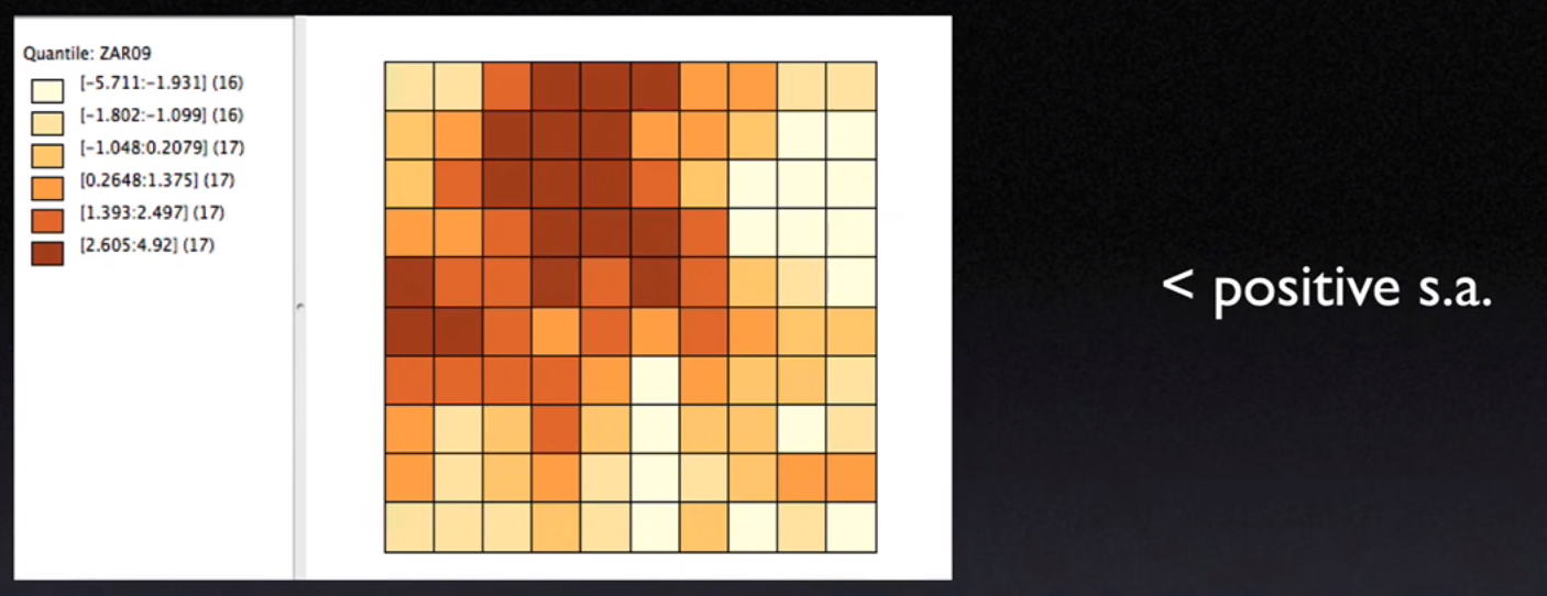
10.2.1. Positive Spatial Autocorrelation#
Impression of clustering
Clumps of like values
Like values can be either high (
hot spots) or low (cold spots)
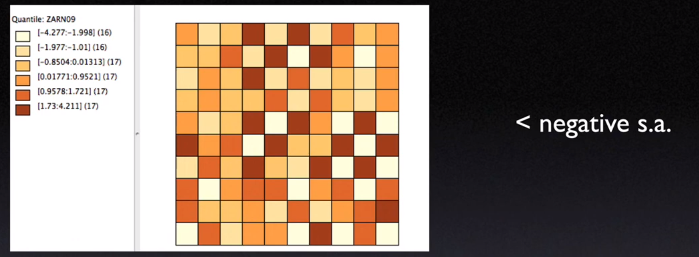
10.2.2. Negative Spatial Autocorrelation#
Checkerboard pattern
Hard to distinguish from spatial randomness
10.3. Spatial Autocorrelation Statistics#
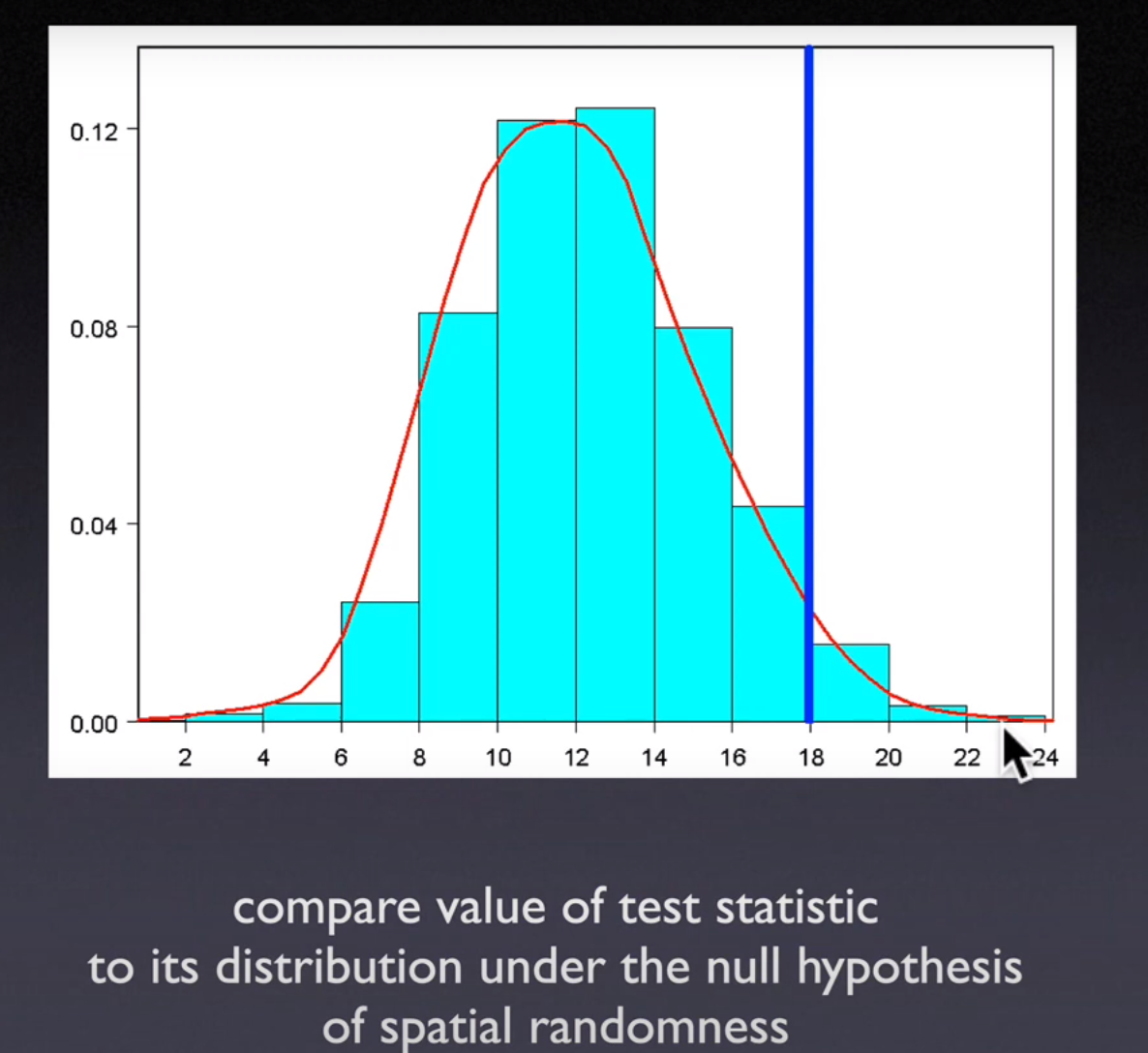
10.3.1. Test Statistics#
Calculated from the data and compared to a reference distribution
How likely is the value if it had occurred under
null hypothesis(spatial randomness)Type-one error:you reject the null hypothesis but it’s trueWhen unlikely (low p-value) the null hypothesis is rejected
10.4. Spatial Autocorrelation Statistic#
Captures both
attribute similarityandlocational similarityAttribute Similarity
Summary of similarity of observations for variable at different locations
Construct \(f(y_i,y_j)\) at location \(i,j\)
10.4.1. Similarity Measure#
Cross product: \(y_i,y_j\)Under randomness (
null hypothesis), cross product is not systematically large or small, otherwise, suggests spatial patterns
10.4.2. Dissimilarity Measure#
Squared difference: \((y_i−y_j )^2\)Absolute difference: \(|y_i−y_j |\)
10.4.3. Locational Similarity#
Formalizing the notion of neighbors \(=(W_ij)\),
spatial weightsWhen are two Spatial units \(i\) and \(j\) a priori likely to interact
Not necessarily a geographical notion, can be based on
social networkorgeneral distanceconcepts
10.5. General Form of Spatial Autocorrelation Statistic#
Sum over all pairs of observations of the product of attribute similarity measure with a neighbor indicator (spatial weight)
\(\sum_{ij}f(x_i,x_j)W_{ij}\)
where \(f(x_i,x_j)\) is
attribute similarity, \(W_ij\) is aspatial weight