16. Convolution Neural Network#
16.1. Introduction#

16.1.1. Single Layer Neural Network#
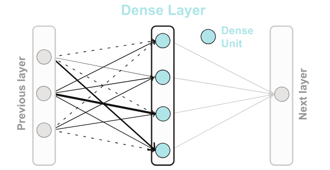
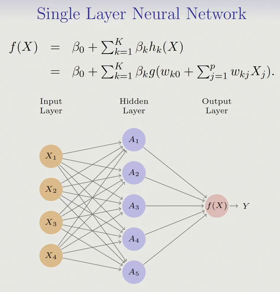
A single-layer neural network, also known as a
perceptron, is one of the simplest forms of artificial neural networks.It consists of only one layer of artificial neurons, also called
nodesorunits, arranged in a single layer.Despite its simplicity, a single-layer neural network can be powerful for solving certain types of problems, particularly those that involve linearly separable data.
In a single-layer neural network, each neuron receives input signals, applies weights to those inputs, sums them up, and then applies an activation function to produce an output.
The output is typically used to make predictions or classify input data into different categories.
16.2. Activation Function:#
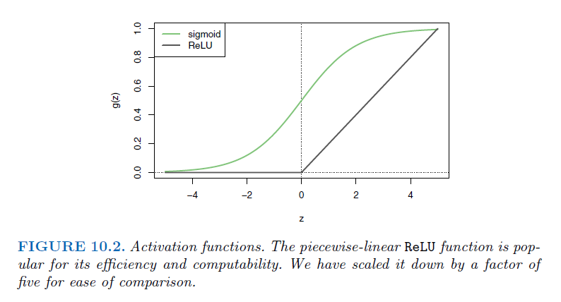
An activation function is a mathematical function applied to the output of each neuron in a neural network. It introduces non-linearity to the network, enabling it to learn complex patterns and relationships in the data.
16.2.1. Purpose#
Non-Linearity: Activation functions introduce non-linear transformations to the input, allowing neural networks to model non-linear relationships in data. Without activation functions, even a multi-layer neural network would behave like a single-layer perceptron, unable to capture complex patterns.
Normalization: They normalize the output of neurons, ensuring that the values fall within a certain range. This can aid in stabilizing and speeding up the training process.
Feature Learning: Activation functions help in learning useful features from the input data, enabling the network to represent and understand the underlying structure of the data.
16.2.2. Common Activation Functions#
ReLU (Rectified Linear Unit):
\(f(x) = max(0,x)\)
ReLU sets all negative values to zero, introducing sparsity and accelerating the learning process.
Widely used due to its simplicity and effectiveness.
Sigmoid
\(f(x) = \frac{1}{1+e^{-x}}\)
S-shaped curve squashes the output between 0 and 1, suitable for binary
classificationtasks.However, it suffers from
vanishing gradient problems.
Tanh (Hyperbolic Tangent)
\(f(x) = \frac{e^x-e^{-x}}{e^x+e^{-x}}\)
Similar to the sigmoid function but maps the output between -1 and 1, addressing the
vanishing gradient problemto some extent.
SoftmaxUsed in the output layer for multi-class classification tasks.
It converts the raw scores into probabilities, ensuring that the sum of probabilities across all classes equals one.
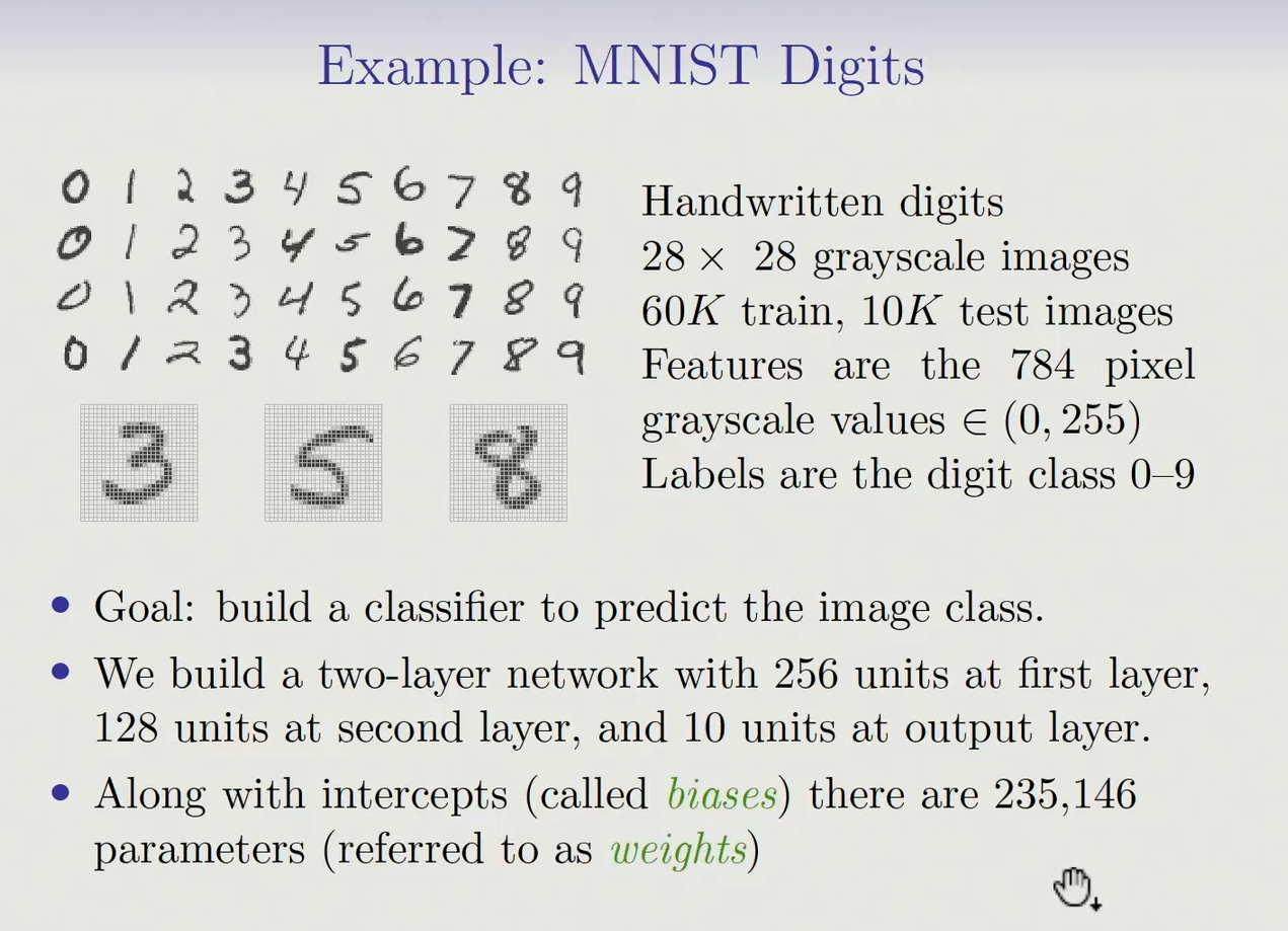
16.4. Example of MNIST Digits#
import tensorflow as tf
from tensorflow.keras import layers, models, datasets
import matplotlib.pyplot as plt
import numpy as np
# Load MNIST dataset
(train_images, train_labels), (test_images, test_labels) = datasets.mnist.load_data()

# Preprocess the data
train_images = train_images.reshape((60000, 28, 28, 1)).astype('float32') / 255
test_images = test_images.reshape((10000, 28, 28, 1)).astype('float32') / 255

# Convert labels to one-hot encoding
train_labels = tf.keras.utils.to_categorical(train_labels)
test_labels = tf.keras.utils.to_categorical(test_labels)
# Define the model
model = models.Sequential([
    layers.Conv2D(256, (3, 3), activation='relu', input_shape=(28, 28, 1)),
    layers.MaxPooling2D((2, 2)),
    layers.Conv2D(128, (3, 3), activation='relu'),
    layers.MaxPooling2D((2, 2)),
    layers.Flatten(),
    # layers.Dense(64, activation='relu'),
    layers.Dense(10, activation='softmax')
])
# Compile the model
model.compile(optimizer='adam',
              loss='categorical_crossentropy',
              metrics=['accuracy'])

# Train the model
history = model.fit(train_images, train_labels, epochs=5, batch_size=64, validation_split=0.2)

# Evaluate the model
test_loss, test_acc = model.evaluate(test_images, test_labels)
print('Test accuracy:', test_acc)
Epoch 1/5
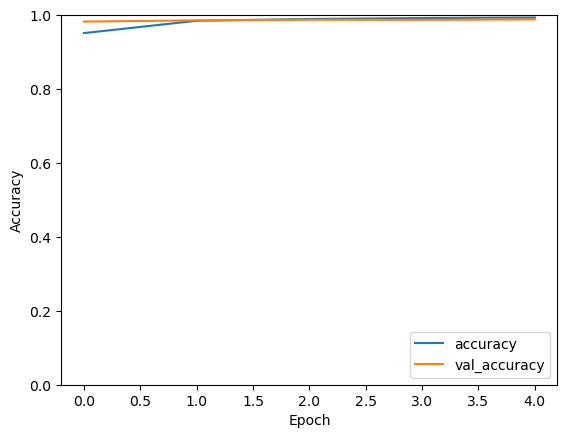
750/750 [==============================] - 10s 6ms/step - loss: 0.1591 - accuracy: 0.9513 - val_loss: 0.0605 - val_accuracy: 0.9825
Epoch 2/5
750/750 [==============================] - 4s 5ms/step - loss: 0.0494 - accuracy: 0.9848 - val_loss: 0.0474 - val_accuracy: 0.9859
Epoch 3/5
750/750 [==============================] - 4s 5ms/step - loss: 0.0346 - accuracy: 0.9896 - val_loss: 0.0427 - val_accuracy: 0.9875
Epoch 4/5
750/750 [==============================] - 4s 5ms/step - loss: 0.0248 - accuracy: 0.9921 - val_loss: 0.0415 - val_accuracy: 0.9872
Epoch 5/5
750/750 [==============================] - 4s 5ms/step - loss: 0.0202 - accuracy: 0.9936 - val_loss: 0.0426 - val_accuracy: 0.9884
313/313 [==============================] - 1s 2ms/step - loss: 0.0357 - accuracy: 0.9890
Test accuracy: 0.9890000224113464
# Plot training history
plt.plot(history.history['accuracy'], label='accuracy')
plt.plot(history.history['val_accuracy'], label = 'val_accuracy')
plt.xlabel('Epoch')
plt.ylabel('Accuracy')
plt.ylim([0, 1])
plt.legend(loc='lower right')
plt.show()
# Randomly pick 10 test images
random_indices = np.random.choice(len(test_images), size=20, replace=False)
random_test_images = test_images[random_indices]
random_test_labels = test_labels[random_indices]

# Predict labels for the random test images
predictions = model.predict(random_test_images)
predicted_labels = np.argmax(predictions, axis=1)

# Plot the images with their true and predicted labels
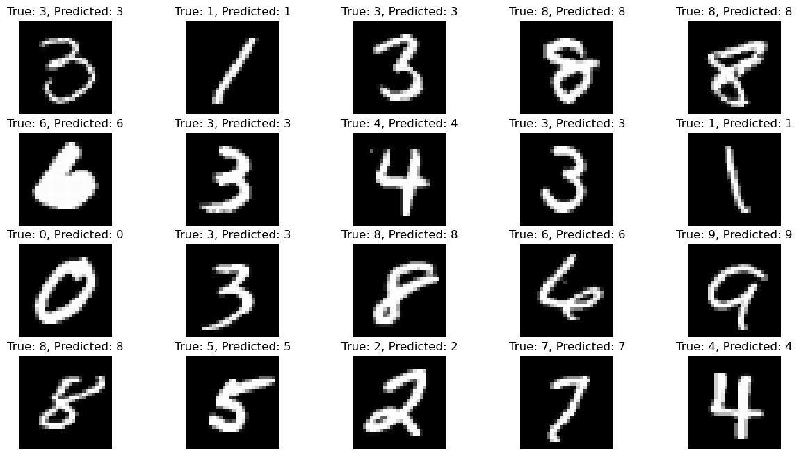
plt.figure(figsize=(15, 8))
for i in range(20):
    plt.subplot(4, 5, i + 1)
    plt.imshow(random_test_images[i].reshape(28, 28), cmap='gray')
    plt.title(f'True: {np.argmax(random_test_labels[i])}, Predicted: {predicted_labels[i]}')
    plt.axis('off')
plt.show()
1/1 [==============================] - 0s 112ms/step
16.5. Convolutional Neural Network (CNN)#
Introduction
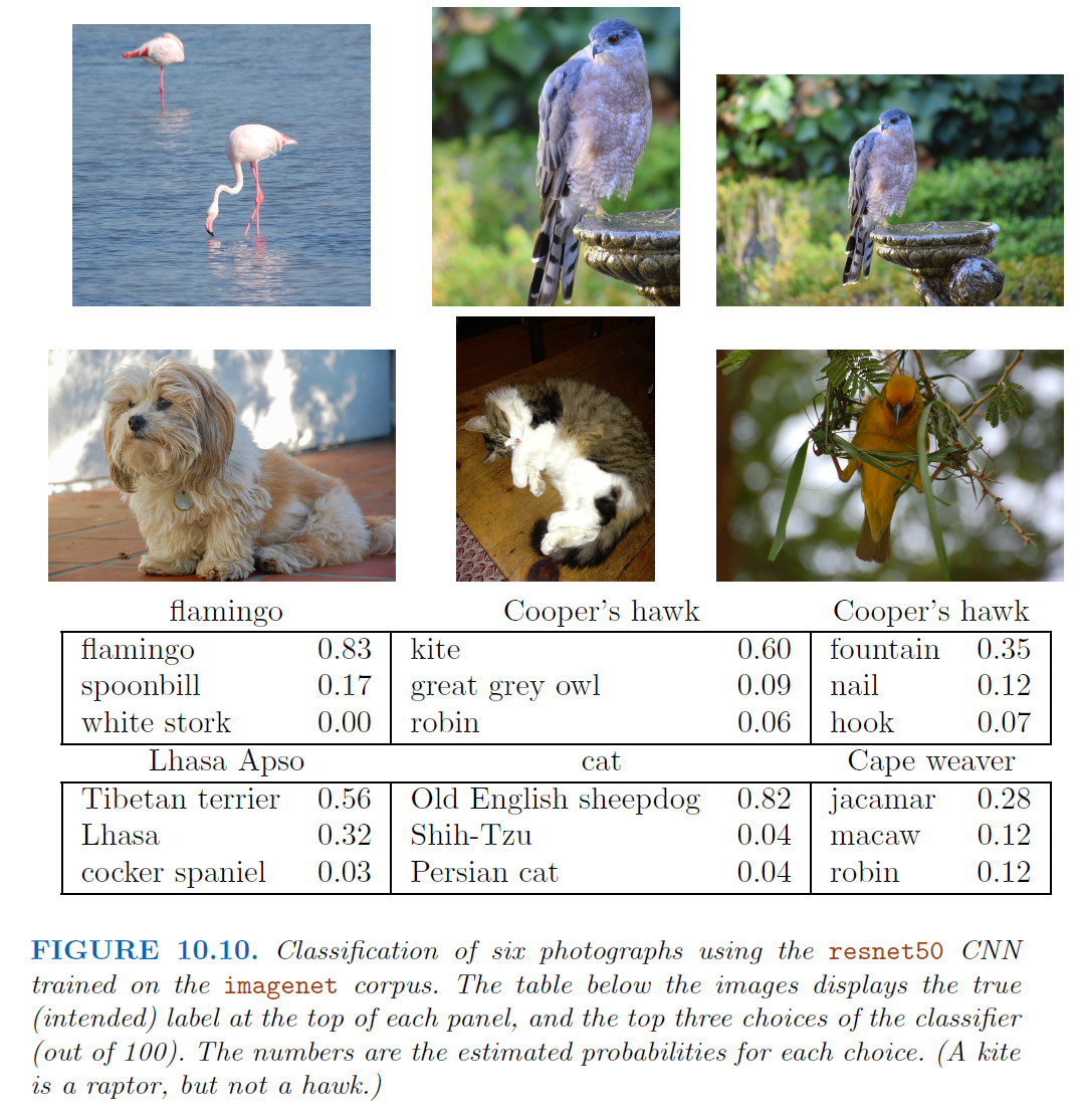
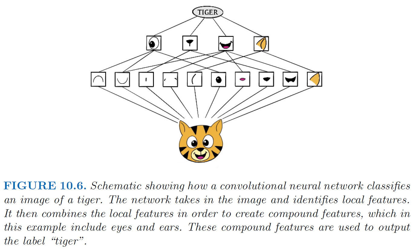
Convolutional Neural Networks (CNNs) are a class of deep learning neural networks, most commonly applied to analyzing visual imagery.
CNNs are particularly effective in tasks such as
image classification,object detection, andimage segmentation.They are inspired by the organization and functioning of the human visual system, with layers of neurons that progressively extract higher-level features from raw pixel values.
16.5.1. Key Components#
Convolutional Layers
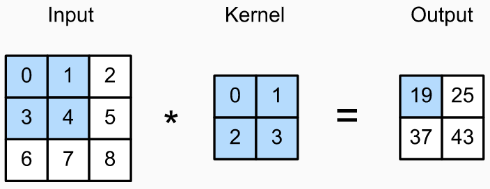
The
convolutional filters(also known askernels) are learned during the training process.Initially, these filters are randomly initialized, and then they are updated iteratively during training through a process called
backpropagation.

Pooling Layers
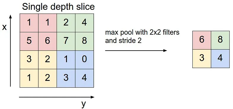
Flatten Layer
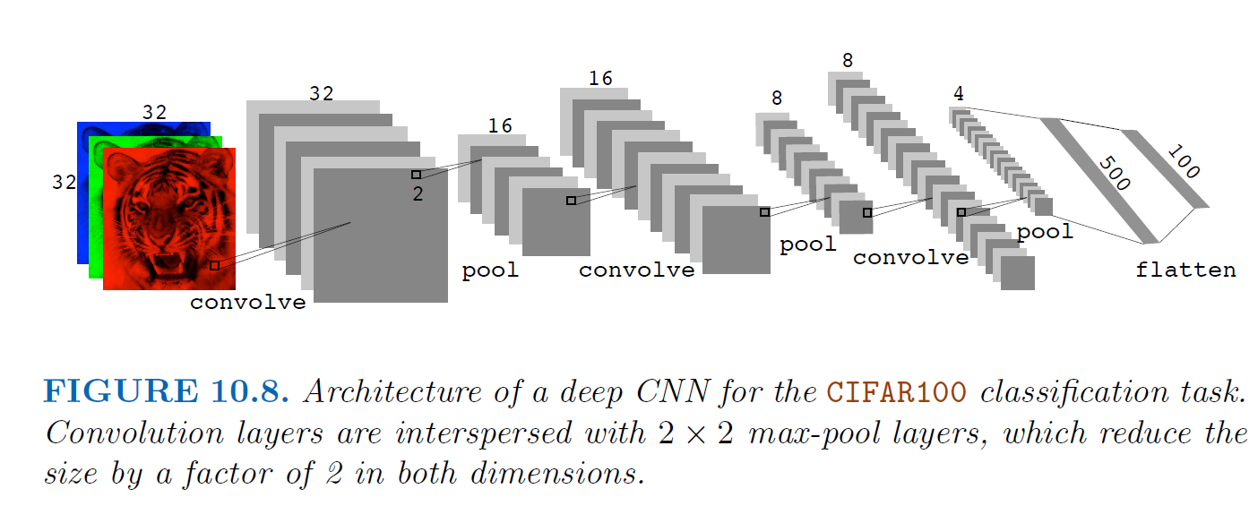
Convolutional Layers usually produce more channels (e.g.
U-NetorRestNet)However, in networks like VGG or AlexNet, the number of channels typically remains constant or decreases as the spatial dimensions of the feature maps increase.
The spatial dimensions of feature maps can change due to
Stride: The stride determines the step size at which the convolutional filter slides over the input image or the preceding layer’s feature map.
A larger stride results in a reduction in the spatial dimensions of the feature map, while a smaller stride preserves more spatial information.
Padding: Padding refers to the addition of extra pixels around the input image or feature map.
It can be used to control the spatial dimensions of the feature map after convolution.

Pooling Layer will not change the number of channels
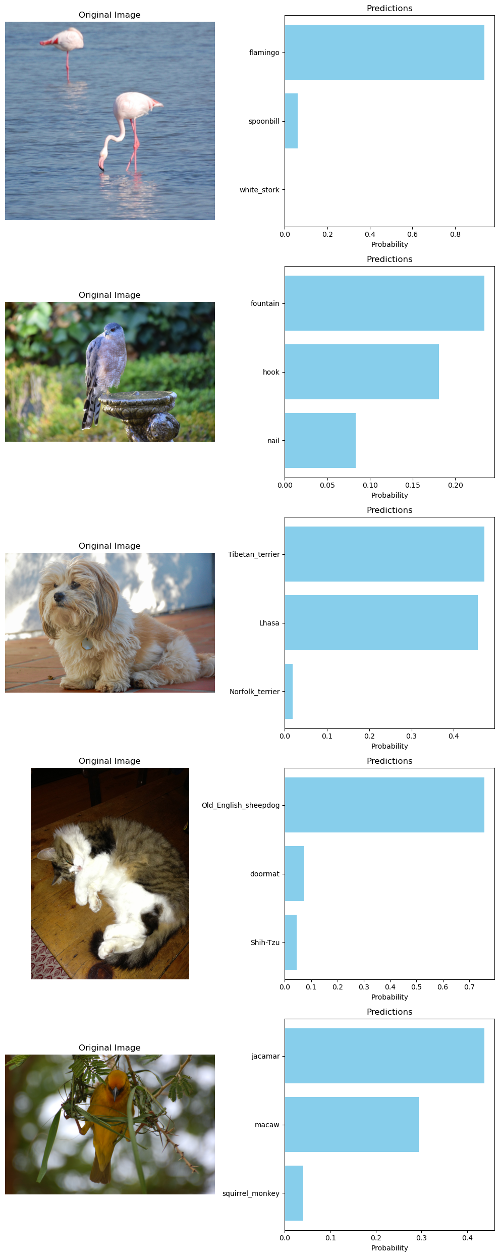
16.5.2. Example of Rest-Net (Pre-trained Model)#
from tensorflow.keras.applications import ResNet50
import os
from tensorflow.keras.preprocessing import image
from tensorflow.keras.applications.resnet50 import preprocess_input, decode_predictions
# Load the pre-trained ResNet50 model
model = ResNet50(weights='imagenet')

# Function to preprocess input image
def preprocess_image(img_array):
    img = tf.image.resize(img_array, (224, 224))
    img_array = np.expand_dims(img, axis=0)
    img_array_copy = img_array.copy()  # Create a writable copy of the array
    return preprocess_input(img_array_copy)

# Function to make predictions
def predict(img_array):
    preprocessed_img = preprocess_image(img_array)
    predictions = model.predict(preprocessed_img)
    decoded_predictions = decode_predictions(predictions, top=3)[0]
    return decoded_predictions

# Path to the directory containing images
image_dir = './Images/'

# Get list of image files in the directory
image_files = [file for file in os.listdir(image_dir) if file.endswith('.jpg') or file.endswith('.png')]

# Plotting images and predictions
num_images = len(image_files)
num_cols = 2  # Two columns: Original Image and Predictions
num_rows = num_images

fig, axes = plt.subplots(num_rows, num_cols, figsize=(10, 5*num_rows))

for i, filename in enumerate(image_files):
    image_path = os.path.join(image_dir, filename)
    img = image.load_img(image_path)
    img_array = image.img_to_array(img)

    # Making predictions
    predictions = predict(img_array)

    # Plotting the image
    axes[i, 0].imshow(img)
    axes[i, 0].set_title('Original Image')
    axes[i, 0].axis('off')

    # Plotting the predictions
    labels = [label for _, label, _ in predictions]
    scores = [score for _, _, score in predictions]
    axes[i, 1].barh(labels, scores, color='skyblue')
    axes[i, 1].invert_yaxis()
    axes[i, 1].set_title('Predictions')
    axes[i, 1].set_xlabel('Probability')

plt.tight_layout()
plt.show()
1/1 [==============================] - 1s 746ms/step
1/1 [==============================] - 0s 24ms/step
1/1 [==============================] - 0s 23ms/step
1/1 [==============================] - 0s 24ms/step
1/1 [==============================] - 0s 26ms/step
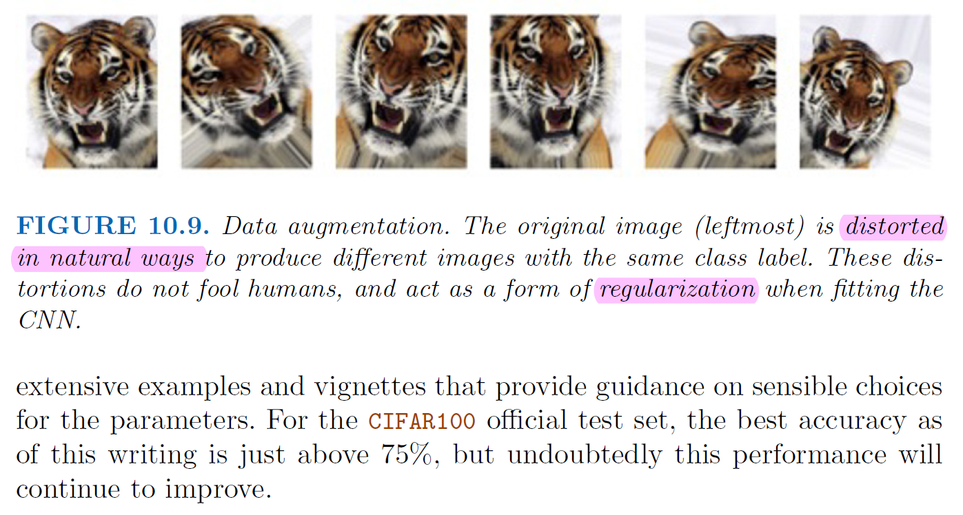
16.5.3. Regularization In CNN#
