Non-linear Regression

7. Non-linear Regression#

The truth is not always linear

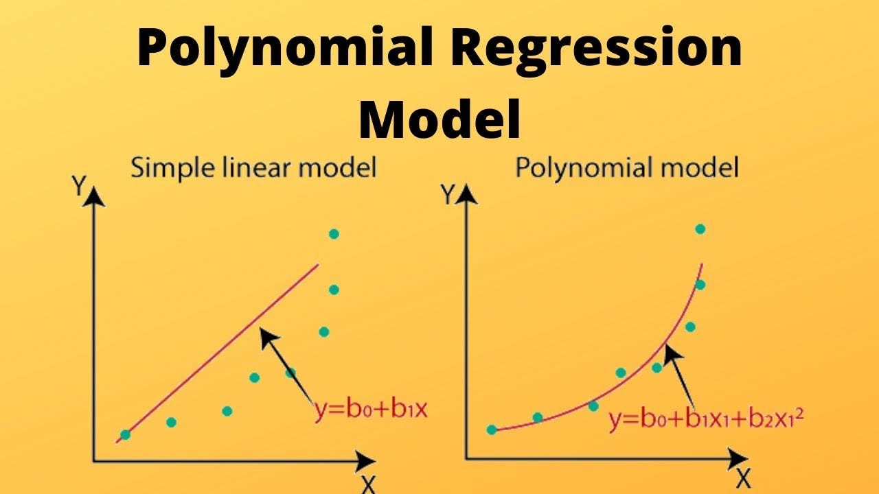
7.1. Polynomial regression#

y_{1} = β_{0} + β_{1} x_{1} + β_{2} x_{1}^{2} + β_{3} x_{1}^{3} + . . . + β_{d} x_{1}^{d} + e

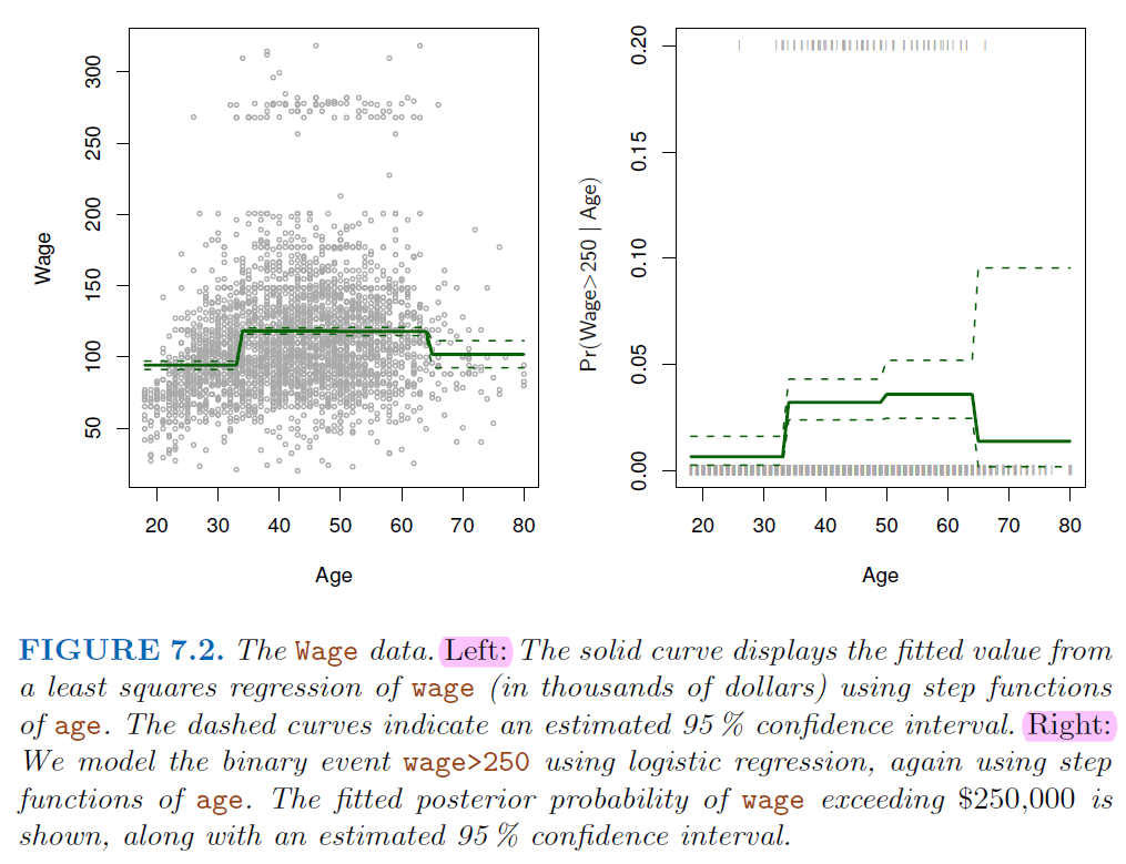
7.2. Step Function#

Using polynomial functions of the features as predictors in a linear model imposes a global structure on the non-linear function of X.
We can instead use step functions in order to avoid imposing such a global structure.
- This amounts to converting a continuous variable into an ordered categorical variable.

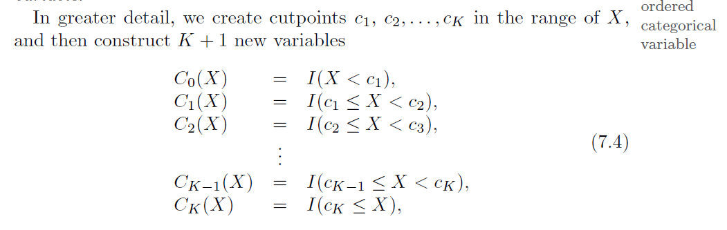
Divide the target variable into discrete classes
- Can use Breakpoint test statistics to help this transforming.

7.3. Break Point Statistics#

Breakpoint checking is a statistical technique used to identify structural changes or breakpoints in data series.
These changes could indicate shifts in underlying processes, trends, or relationships within the data.

7.3.1. Chow Test#

The chow test statistic is calculated as follows:
- $R S S_{r}$ is the residual sum of squares from the model with all data combined.
- $R S S_{1}$ and $R S S_{2}$ are the residual sum of squares from the separate models for each segment.
- $k$ is the number of parameters estimated in each segment.
- $n_{1}$ and $n_{2}$ are the number of observations in each segment $ $F = \frac{R S S_{r} - (R S S_{1} + R S S_{2}) / k}{(R S S_{1} + R S S_{2}) / (n_{1} + n_{2} - 2 k)}$ $

import numpy as np
import statsmodels.api as sm
import matplotlib.pyplot as plt

# Generate two sections of data with different linear functions
np.random.seed(0)

# First section
n1 = 50
x1 = np.linspace(0, 5, n1)
y1 = 2 * x1 + np.random.normal(0, 1, n1)

# Second section
n2 = 50
x2 = np.linspace(5, 10, n2)
y2 = 3 * x2 + np.random.normal(0, 1, n2)

# Merge the sections
x = np.concatenate([x1, x2])
y = np.concatenate([y1, y2])

# Initialize variables to store best breakpoint and test statistic
best_breakpoint = None
best_F = 0

# Iterate over potential breakpoints
for i in range(1, len(x)-1):
    x1 = x[:i]
    y1 = y[:i]
    x2 = x[i:]
    y2 = y[i:]
    
    # Fit model with all data combined
    X_combined = sm.add_constant(np.concatenate([x1, x2]))
    model_combined = sm.OLS(np.concatenate([y1, y2]), X_combined).fit()
    RSS_r = model_combined.ssr
    k = 2  # Number of parameters estimated in each segment
    
    # Fit separate models for each segment
    model1 = sm.OLS(y1, sm.add_constant(x1)).fit()
    model2 = sm.OLS(y2, sm.add_constant(x2)).fit()
    RSS_1 = model1.ssr
    RSS_2 = model2.ssr
    n1 = len(x1)
    n2 = len(x2)
    
    # Calculate Chow test statistic
    F_chow = ((RSS_r - (RSS_1 + RSS_2)) / k) / ((RSS_1 + RSS_2) / (n1 + n2 - 2*k))
    
    # Update best breakpoint if necessary
    if F_chow > best_F:
        best_F = F_chow
        best_breakpoint = i

# Visualize results
plt.figure(figsize=(10, 6))
plt.scatter(x, y, label='Data')
plt.axvline(x=x[best_breakpoint], color='r', linestyle='--', label=f'Best Breakpoint at {x[best_breakpoint]:.2f}')
plt.xlabel('x')
plt.ylabel('y')
plt.title('Chow Test: Best Breakpoint')
plt.legend()
plt.grid(True)
plt.show()

print("Best Breakpoint:", x[best_breakpoint])
print("Chow Test Statistic:", best_F)

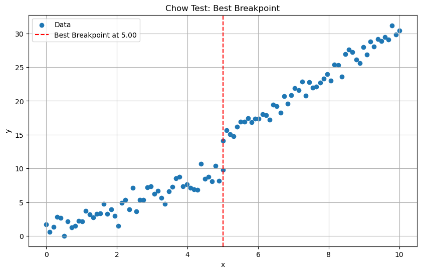
../../_images/fc23481b98f8fe9f77e91081e7ff5627066efe76fba981543583cbfb7b0590a1.png

Best Breakpoint: 5.0
Chow Test Statistic: 157.58585701856043

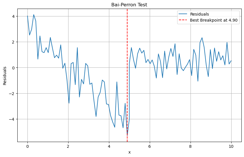
7.3.2. Bai-Perron Test#

It uses a dynamic programming approach to efficiently identify the number and locations of breakpoints by minimizing the sum of squared residuals.
Steps:
1. Let $y_{t} = X_{t}^{T} β_{j} + ε_{t}$ be the linear regression model with $m$ breakpoints
2. sup $F_{T} (λ_{1}, . . ., λ_{m})$ , where $λ_{j} = T_{j} / T$ are the breakpoint fractions
  - And $F_{T}$ is a function of the sum of squared residuals for different partitions of the sample.

from statsmodels.stats.diagnostic import breaks_cusumolsresid

# Fit the model
X_combined = sm.add_constant(x)
model_combined = sm.OLS(y, X_combined).fit()
residuals = model_combined.resid

# Perform Bai-Perron Test
breakpoints = breaks_cusumolsresid(residuals)

# Visualize Bai-Perron Test
plt.figure(figsize=(10, 6))
plt.plot(x, residuals, label='Residuals')
plt.axvline(x=x[np.argmin(residuals)], color='r', linestyle='--', label=f'Best Breakpoint at {x[np.argmin(residuals)]:.2f}')
plt.xlabel('x')
plt.ylabel('Residuals')
plt.title('Bai-Perron Test')
plt.legend()
plt.grid(True)
plt.show()

# print("Detected Breakpoints:", [x[bp] for bp in breakpoints])

../../_images/0ed93a6abe5f6f56373045f3821e7a62dc60659cfa8e1be5905ca7580b4680e5.png

7.4. Regression Splines#

7.4.1. Piecewise Polynomials#

Step function + Polynomials regression

Put the constraint on Piecewise Cubic
- Green line (2nd plot) force the function to be continuous
- Red line (3rd plot) add constraint of 2nd derivatives (convex)

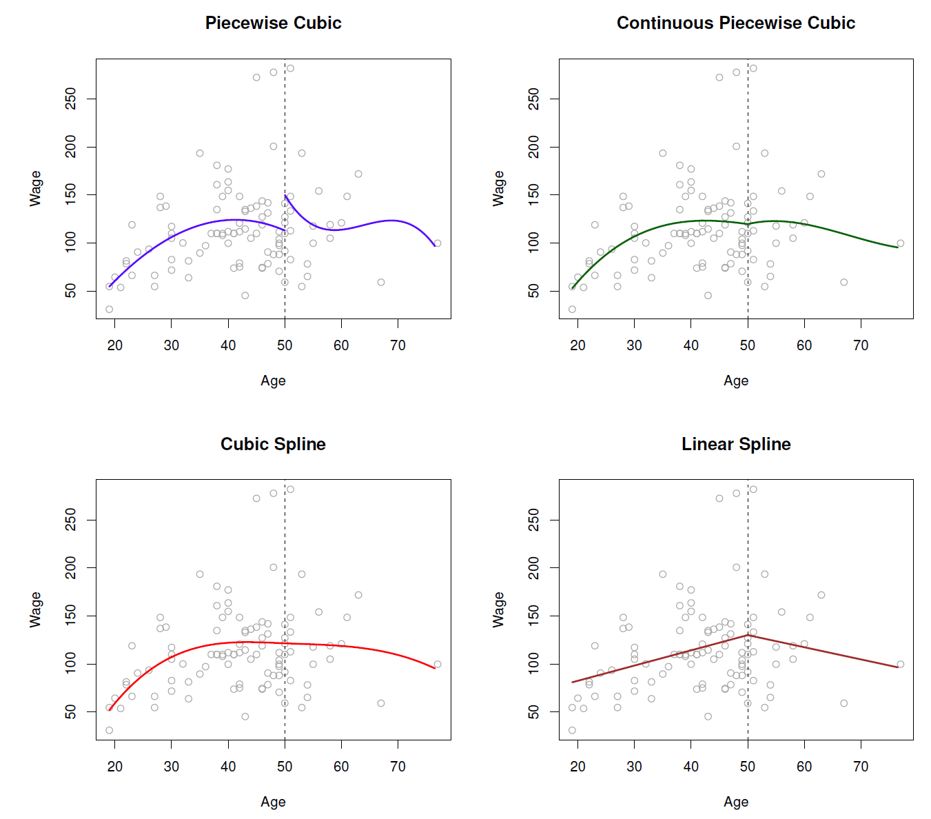
7.4.2. Liner Splines#

A linear spline with knots at $k = 1, . . ., K$ is a piecewise linear polynomial continuous at each knot.
- where the $b_{k}$ are basis functions $ $y_{i} = β_{0} + β_{1} b_{1} (x_{i}) + β_{2} b_{2} (x_{i}) + . . . + β_{K} b_{K} (x_{i}) + e_{i}$ $

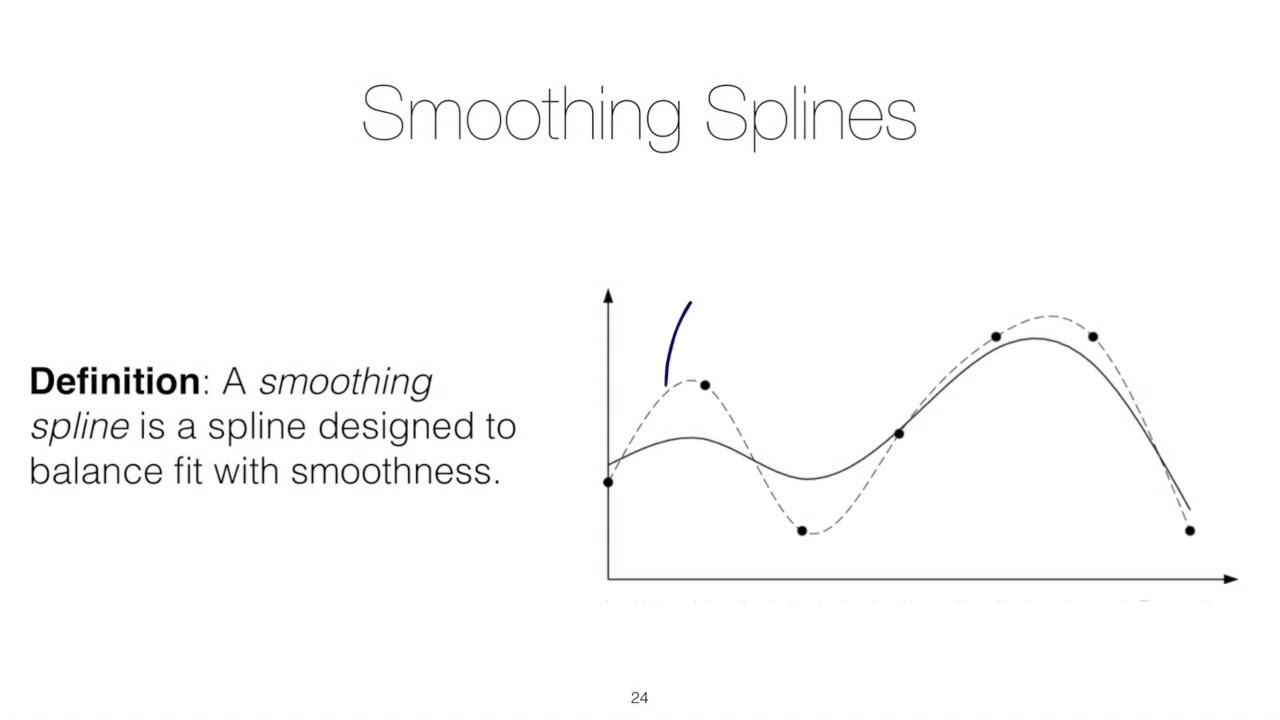
7.4.3. Smoothing Splines#

It consider the following criterion for fitting a smooth function $g (x)$ to data:
- The first term is RSS, and try to make $g (x)$ match the data at each $x$
- The second term is 2nd derivatives, it constraint the smoothness * $λ$ is the tuning parameter, when $λ$ goes infinity, the 2nd derivatives has to be 0, which means a linear function （No Concave-Convexity） $ $m i n i m i z e_{g \in S} \sum_{i = 1}^{n} (y_{i} - g (x_{i}))^{2} + λ \int g^{″} (t)^{2} d t$ $

Non-linear Regression

Contents

7. Non-linear Regression#

7.1. Polynomial regression#

7.2. Step Function#

7.3. Break Point Statistics#

7.3.1. Chow Test#

7.3.2. Bai-Perron Test#

7.4. Regression Splines#

7.4.1. Piecewise Polynomials#

7.4.2. Liner Splines#

7.4.3. Smoothing Splines#

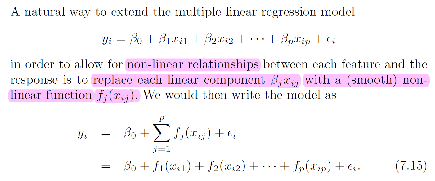
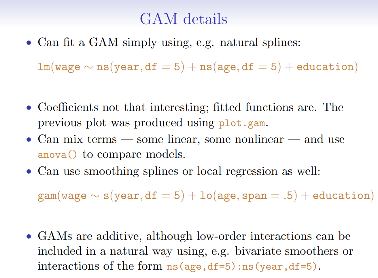
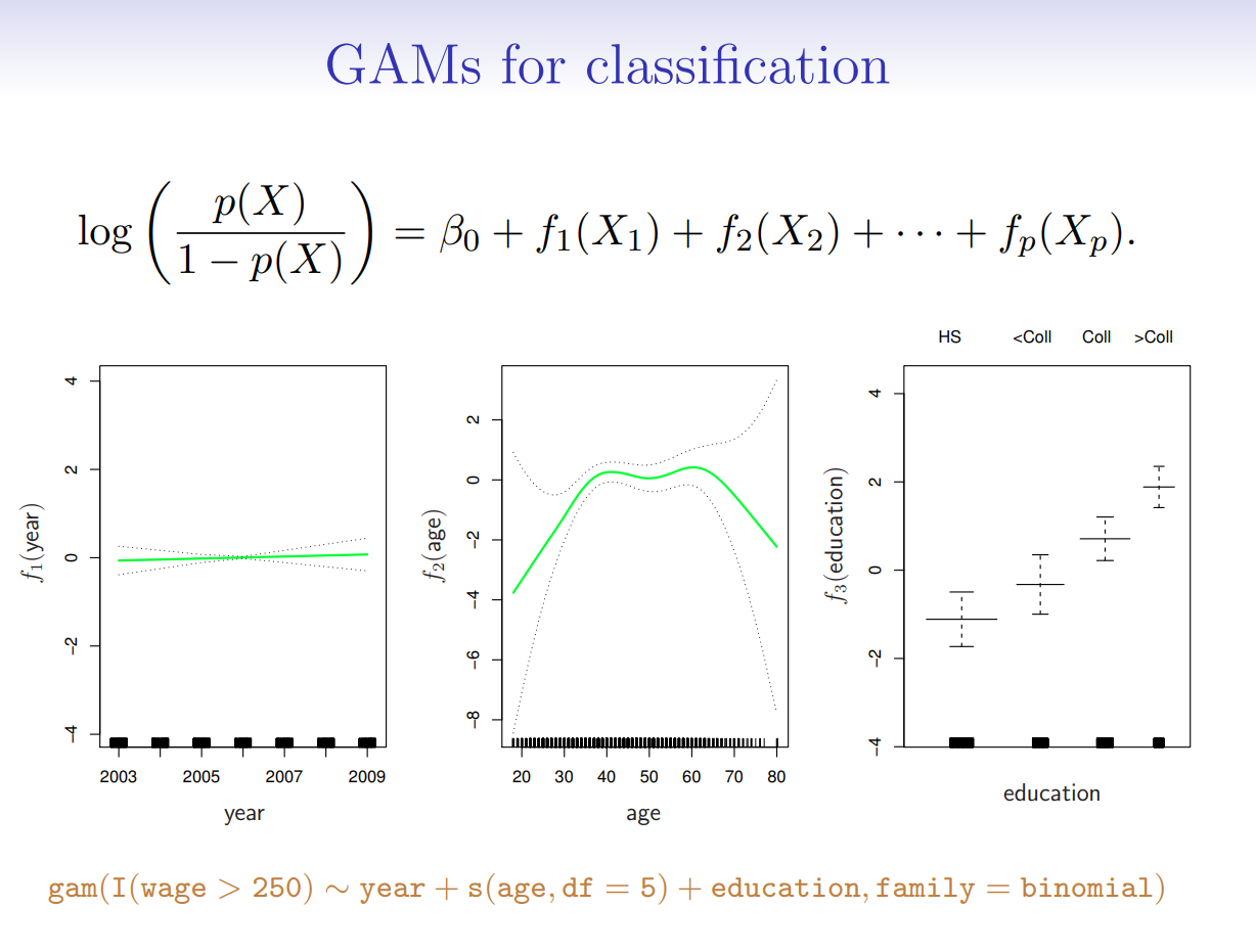
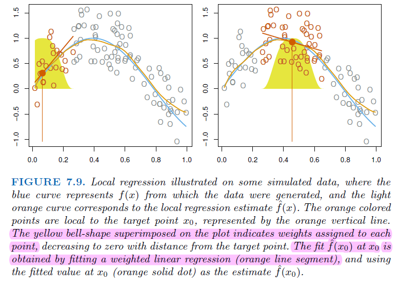
7.5. Generalized Additive Models and Local Regression#

7.5.1. Local Regression#

7.5.2. Generalized Additive Models#