Gradient Descent (GD)

11. Gradient Descent (GD)#

Learning Material for Differential
Learning Material for Linear Algbra
Learning Material for Linear Algbra (Video)

11.1. Introduction to Gradient Descent#

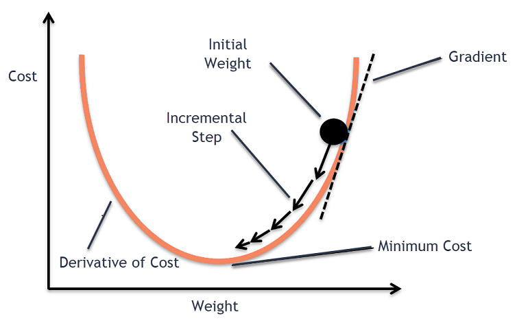
Gradient Descent is an optimization algorithm used to minimize a function by iteratively moving in the direction of steepest descent. It is widely used in machine learning to minimize the cost function.

The basic idea is to update the parameters (weights) of a model in the opposite direction of the gradient of the cost function with respect to the parameters.

11.2. Stochastic Gradient Descent (SGD)#

Reference

Stochastic Gradient Descent (SGD) is a variant of gradient descent where, instead of computing the gradient of the entire dataset, we compute the gradient of the cost function with respect to the parameters based on a single training example at each iteration. * This makes SGD much faster and more scalable, especially for large datasets.

11.2.1. General algorithm for implementing SGD#

Initialize the model parameters randomly or with some predefined values.
Shuffle the training dataset.
For each training example:

Compute the gradient of the cost function with respect to the parameters using the current training example.
Update the parameters in the direction opposite to the gradient by a small step size (learning rate).

Repeat the process until convergence or for a fixed threshold of iterations.

11.3. Example: Linear Regression with GD#

11.3.1. Simulate linear regression data#

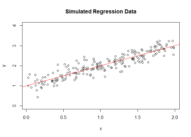
y = 1 + x + e, where e ~ normal(0,0.25)

set.seed(1)
b0 <- 1; b1 <- 1; n <- 200
x <- runif(n,0,2)
y <- b0 + b1*x + rnorm(n, sd=0.25)
summary(lm(y~x))

## 
## Call:
## lm(formula = y ~ x)
## 
## Residuals:
##      Min       1Q   Median       3Q      Max 
## -0.72323 -0.15560 -0.01819  0.16244  0.66273 
## 
## Coefficients:
##             Estimate Std. Error t value Pr(>|t|)    
## (Intercept)  1.00136    0.03831   26.14   <2e-16 ***
## x            0.99771    0.03285   30.37   <2e-16 ***
## ---
## Signif. codes:  0 '***' 0.001 '**' 0.01 '*' 0.05 '.' 0.1 ' ' 1
## 
## Residual standard error: 0.2493 on 198 degrees of freedom
## Multiple R-squared:  0.8233, Adjusted R-squared:  0.8224 
## F-statistic: 922.4 on 1 and 198 DF,  p-value: < 2.2e-16

plot the dataset

plot(y~x, ylim=c(0,4), main="Simulated Regression Data")
abline(lm(y~x), col="red")

11.3.2. Define loss function and gradient search function#

Loss function in torch

In this example, we use MSE (squared L2 norm) as our loss function, we ignore n since it will not change the optimum solution position

$MSE = \frac{1}{n}\sum(y-\hat y)^2=\frac{1}{n}\sum(y-(\hat \beta_0+\hat \beta_1x))^2$

##
lossFct <- function(y,x,b0,b1){
  sum((y-(b0+b1*x))^2)
} #end::lossFct

To minimize the MSE, we use gradient descent. The gradient of the MSE with respect to the parameters β̂₀ and β̂₁ are computed as follows:

More Info

\[ \frac{\partial f}{\partial \hat \beta_0} = -\frac{2}{n}\sum_i(y_i-(\hat \beta_0+\hat \beta_1x_i)) \]

\[ \frac{\partial f}{\partial \hat \beta_1} = -\frac{2}{n}\sum_ix_i(y_i-(\hat \beta_0+\hat \beta_1x_i)) \]

Then, we move the current estimated parameter β₀ and β₁ to the opposite direction of gradients by α (also called learning rate) steps, here is the equation $$ \hat \beta_0^{new}=\hat \beta_0^{old} - \frac{\partial f}{\partial \hat \beta_0} \* \alpha $$

\[ \hat \beta_1^{new}=\hat \beta_1^{old} - \frac{\partial f}{\partial \hat \beta_1}\* \alpha \]

gradientUpdateFct <- function(y, x, b0Old, b1Old, alpha) {
  # The objective is to move to a minimum loss

  # Compute the derivative of the loss function with respect to b0
  derivb0 <- -2 * sum((y - (b0Old + b1Old * x)))    # at optimum equal to zero
  
  # Compute the derivative of the loss function with respect to b1
  derivb1 <- -2 * sum(x * (y - (b0Old + b1Old * x)))  # at optimum equal to zero
  
  # Update the parameters b0 and b1 using the gradients and learning rate alpha
  b0New <- b0Old - derivb0 * alpha / length(x)
  b1New <- b1Old - derivb1 * alpha / length(x)
  
  # Return the updated parameters as a vector
  return(c(b0New, b1New))
}

11.3.3. Start Iteration#

In this example, we set * alpha (learning rate) as 0.05 * treshold as 0.0005 * maxIter as 200

We can start β̂₀ and β̂₁ randomly, but for visualization purpose, we set both as 0 at first

## Set parameters controlling the gradient descent search and history
b0 <- 0; b1 <- 0             # Set starting values
loss <- lossFct(y, x, b0, b1)   # Loss at start
threshold <- 0.0005          # Change in the loss for gradient descent
alpha <- 0.05                # Learning rate: update step length
maxIter <- 200               # Maximum iterations for gradient descent

plot(y ~ x, ylim = c(0, 4), main = "Simulated Regression Data")
abline(lm(y ~ x), col = "red")

## Start iterative search
abline(a = b0, b = b1, col = "green")  # Starting regression line
i <- 1
iterHist <- rbind(NULL, c(i, b0, b1, loss))
lossOld <- Inf

while (abs(lossOld - loss) > threshold) {
  i <- i + 1
  lossOld <- loss
  b <- gradientUpdateFct(y, x, b0, b1, alpha)
  b0 <- b[1]
  b1 <- b[2]
  loss <- lossFct(y, x, b0, b1)
  iterHist <- rbind(iterHist, c(i, b0, b1, loss))

  if ((i %% 5) == 0) {  # Plot results of every 5th iteration
    abline(a = b0, b = b1, col = "green")  # Updated regression line
    cat("Iteration:", i, "| Estimated Beta_0:", round(b0, 4), "| Estimated Beta_1:", round(b1, 4), "| Loss:", round(loss, 4), "\n")
    if (i > maxIter) break
    Sys.sleep(0.5)  # Slow down for visualization
  }  # end::if
}  # end::while

## Iteration: 5 | Estimated Beta_0: 0.581 | Estimated Beta_1: 0.6809 | Loss: 130.0938 
## Iteration: 10 | Estimated Beta_0: 0.8234 | Estimated Beta_1: 0.9576 | Loss: 22.0329 
## Iteration: 15 | Estimated Beta_0: 0.8957 | Estimated Beta_1: 1.0328 | Loss: 13.34 
## Iteration: 20 | Estimated Beta_0: 0.9197 | Estimated Beta_1: 1.0512 | Loss: 12.6129 
## Iteration: 25 | Estimated Beta_0: 0.9297 | Estimated Beta_1: 1.0537 | Loss: 12.5278 
## Iteration: 30 | Estimated Beta_0: 0.9356 | Estimated Beta_1: 1.0518 | Loss: 12.4974 
## Iteration: 35 | Estimated Beta_0: 0.9402 | Estimated Beta_1: 1.0488 | Loss: 12.4743 
## Iteration: 40 | Estimated Beta_0: 0.9441 | Estimated Beta_1: 1.0458 | Loss: 12.4542 
## Iteration: 45 | Estimated Beta_0: 0.9477 | Estimated Beta_1: 1.0428 | Loss: 12.4366 
## Iteration: 50 | Estimated Beta_0: 0.9511 | Estimated Beta_1: 1.0399 | Loss: 12.4212 
## Iteration: 55 | Estimated Beta_0: 0.9543 | Estimated Beta_1: 1.0373 | Loss: 12.4076 
## Iteration: 60 | Estimated Beta_0: 0.9573 | Estimated Beta_1: 1.0348 | Loss: 12.3957 
## Iteration: 65 | Estimated Beta_0: 0.96 | Estimated Beta_1: 1.0325 | Loss: 12.3853 
## Iteration: 70 | Estimated Beta_0: 0.9626 | Estimated Beta_1: 1.0303 | Loss: 12.3761 
## Iteration: 75 | Estimated Beta_0: 0.9651 | Estimated Beta_1: 1.0282 | Loss: 12.368 
## Iteration: 80 | Estimated Beta_0: 0.9674 | Estimated Beta_1: 1.0263 | Loss: 12.361 
## Iteration: 85 | Estimated Beta_0: 0.9695 | Estimated Beta_1: 1.0245 | Loss: 12.3547 
## Iteration: 90 | Estimated Beta_0: 0.9715 | Estimated Beta_1: 1.0228 | Loss: 12.3493 
## Iteration: 95 | Estimated Beta_0: 0.9734 | Estimated Beta_1: 1.0212 | Loss: 12.3445 
## Iteration: 100 | Estimated Beta_0: 0.9751 | Estimated Beta_1: 1.0198 | Loss: 12.3403 
## Iteration: 105 | Estimated Beta_0: 0.9768 | Estimated Beta_1: 1.0184 | Loss: 12.3366 
## Iteration: 110 | Estimated Beta_0: 0.9783 | Estimated Beta_1: 1.0171 | Loss: 12.3333 
## Iteration: 115 | Estimated Beta_0: 0.9798 | Estimated Beta_1: 1.0159 | Loss: 12.3305

abline(lm(y ~ x), col = "red")  # Plot final regression line again

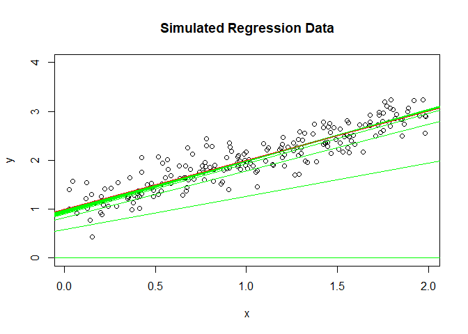
cat("\nFinal solution gradient descent\nBeta_0:", round(iterHist[nrow(iterHist), 2], 4), "| Beta_1:", round(iterHist[nrow(iterHist), 3], 4), "\n")

## 
## Final solution gradient descent
## Beta_0: 0.9809 | Beta_1: 1.0149

It convergence before 200 round iterations.

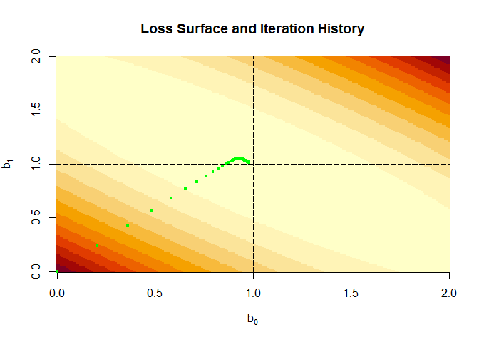
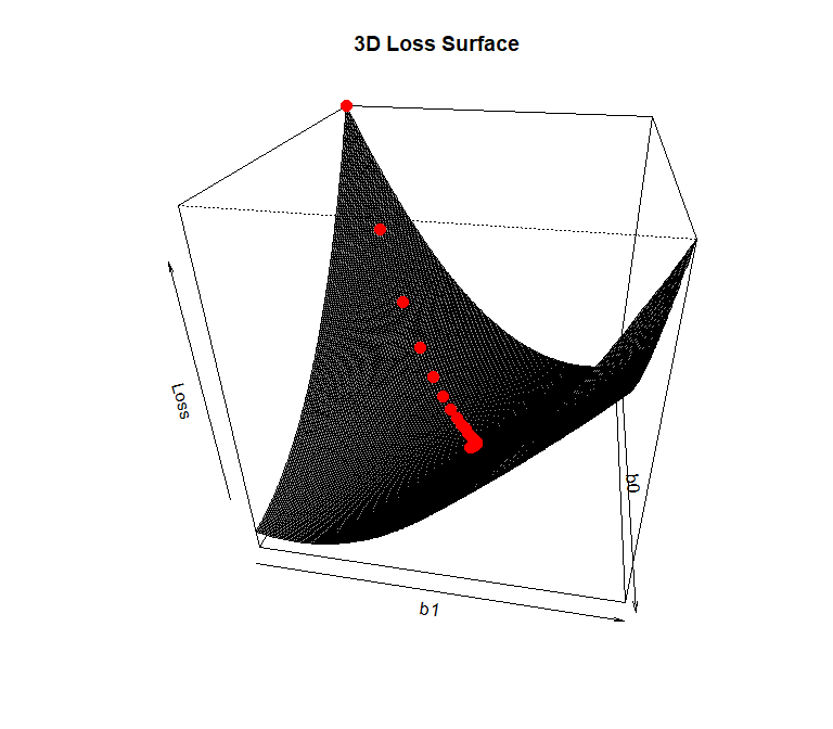
11.3.4. Visualize the loss surface#

b0Grid <- seq(0,2, by=0.01)
b1Grid <- seq(0,2, by=0.01)

##
## Setup loss surface
##
lossValMat <- matrix(NA, nrow = length(b0Grid), ncol = length(b1Grid))
for (i in 1:length(b0Grid)) {
  for (j in 1:length(b1Grid)) {
    lossValMat[i, j] <- lossFct(y, x, b0Grid[i], b1Grid[j])
  }
}

##
## Plot loss surface and iteration history
##
image(b0Grid, b1Grid, lossValMat, ,xlab=expression(b[0]),ylab=expression(b[1]),
      main="Loss Surface and Iteration History")
abline(v=coef(lm(y~x))[1], h=coef(lm(y~x))[2], lty="longdash")
points(iterHist[1:nrow(iterHist),2:3], pch=".", cex=4, col="green")

b0Grid <- seq(0, 2, by = 0.01)
b1Grid <- seq(0, 2, by = 0.01)

lossValMat <- matrix(NA, nrow = length(b0Grid), ncol = length(b1Grid))
for (i in 1:length(b0Grid)) {
  for (j in 1:length(b1Grid)) {
    lossValMat[i, j] <- lossFct(y, x, b0Grid[i], b1Grid[j])
  }
}

# Create the 3D plot
persp3D <- persp(b0Grid, b1Grid, lossValMat, theta = 100, phi = 30,
      xlab = "b0", ylab = "b1", zlab = "Loss",
      main = "3D Loss Surface", shade = 0.75, # Adjust shading for better visibility
      box = TRUE)  # Add a box around the plot

trans3d <- trans3d(x = iterHist[, 2], y = iterHist[, 3], z = iterHist[, 4],
                   pmat = persp3D)
points(trans3d, pch = 19, col = "red", cex = 1.5)

11.4. Example with SGD#

The process is very similar to GD, but we do not compute the gradients from whole dataset, but from samples

set.seed(123)

epochs <- 20          # number of steps

b0Old <- 0;  b1Old <- 0  # Start values for coefficients

for (i in 1:epochs){
  jSeq <- sample(1:n,size = 20)    # Random sequence of observations
  for (j in jSeq){
    b <- gradientUpdateFct(y[j],x[j],b0Old,b1Old,alpha)
    b0Old <- b[1]
    b1Old <- b[2]
  } # end::oneLine
} # end::epoch


cat("\nFinal solution single observation:
    b0: ", b0Old, "b1: ", b1Old,"\n")

## 
## Final solution single observation:
##     b0:  1.040424 b1:  0.9717855