Regression

2. Regression#

2.1. Simple Linear Regression#

$Y = β_{0} + β_{1} x + e$

$Y$ represents the dependent variable or the variable we are trying to predict or explain.
$x$ represents the independent variable or the predictor variable.
$β_{0}$ is the intercept of the regression line, which is the predicted value of $Y$ when $x$ is zero.
$β_{1}$ is the slope of the regression line, representing the average change in $Y$ for a one-unit change in $x$ .
$e$ stands for the error term (also known as the residual), which is the difference between the observed values and the values predicted by the model.

# Import necessary libraries
import numpy as np
from sklearn.linear_model import LinearRegression
import matplotlib.pyplot as plt

# Generate some random data for demonstration
np.random.seed(0) # Seed for reproducibility
x = np.random.rand(100, 1) # 100 random numbers for independent variable
y = 2 + 3 * x + np.random.randn(100, 1) # Dependent variable with some noise

# Create a linear regression model
model = LinearRegression()

# Fit the model with our data (x - independent, y - dependent)
model.fit(x, y)

# Print the coefficients
print("Intercept (beta_0):", model.intercept_)
print("Slope (beta_1):", model.coef_)

Intercept (beta_0): [2.22215108]
Slope (beta_1): [[2.93693502]]

# Use the model to make predictions
y_pred = model.predict(x)

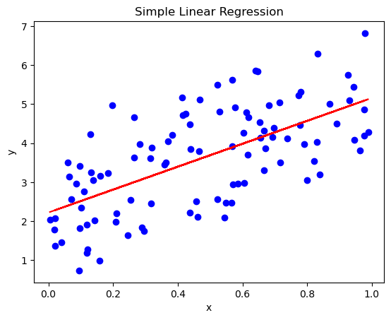
# Plotting
plt.scatter(x, y, color='blue') # actual data points
plt.plot(x, y_pred, color='red') # our model's predictions
plt.title('Simple Linear Regression')
plt.xlabel('x')
plt.ylabel('y')
plt.show()

../../_images/1831aafd86aa4f5485189a6e0ce102e4fa2c052916aacc37e9cac78a7e00ab36.png

2.1.1. Find Best estimator of $β_{1}$ #

2.1.1.1. Ordinary Least Squares#

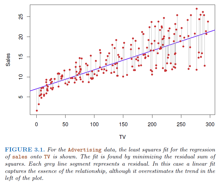
The goal is to find the values of $β_{0}$ and $β_{1}$ that minimize the sum of the squared differences (residuals) between the observed values and the values predicted by the linear model.
$M i n i m i z e (e) = (\sum (y_{i} - (β_{0} + β_{1} x_{i}))^{2})$ , where $y_{i}$ and $x_{i}$ are the observed values.
Steps to calculate it

Calculate the partial derivatives of intercept $β_{0}$ and let it equal to 0
- $\frac{\partial e}{\partial β_{0}} = \sum_{i} 2 (y_{i} - β_{0} - β_{i} x_{i}) (- 1) = 0$
- $\frac{\partial e}{\partial β_{0}} = \sum_{i} β_{1} x_{i} - n * β_{0} - \sum_{i} y_{i} = 0$
- $\sum_{i} β_{1} x_{i} + n * β_{0} - \sum_{i} y_{i} = 0 \to n * β_{1} \bar{x} + n * β_{0} - n * \bar{y} = 0$
- $n * β_{1} \bar{x} + n * β_{0} - n \* \bar{y} = 0 \to β_{1} \bar{x} + β_{0} - \bar{y} = 0$
- $β_{1} \bar{x} + β_{0} - \bar{y} = 0 \to β_{0} = \bar{y} - β_{1} \bar{x}$
Calculate the partial derivative of slope $β_{1}$ and let it equal to 0
- $\frac{\partial e}{\partial β_{1}} = \sum_{i} 2 (y_{i} - β_{1} x_{i} - β_{0}) (- x_{i}) = 0$
- $\sum_{i} 2 (y_{i} - β_{1} x_{i} - β_{0}) (- x_{i}) = 0 \to \sum_{i} (β_{1} x_{i}^{2} + β_{0} x_{i} - x_{i} y_{i}) = 0$
- Replace $β_{0}$ with $(\bar{y} - β_{1} \bar{x})$ : $\sum_{i} (β_{1} x_{i}^{2} + (\bar{y} - β_{1} \bar{x}) x_{i} - x_{i} y_{i}) = 0$
- $β_{1} (\sum_{i} x_{i} y_{i} - \bar{y} \sum_{i} x_{i}) = \sum_{i} x_{i}^{2} - \bar{x} \sum_{i} x_{i} \to β_{1} = \frac{\sum_{i} x_{i} y_{i} - \bar{y} \sum_{i} x_{i}}{\sum_{i} x_{i}^{2} - \bar{x} \sum_{i} x_{i}}$
- According to the Summation Property (As shown below):
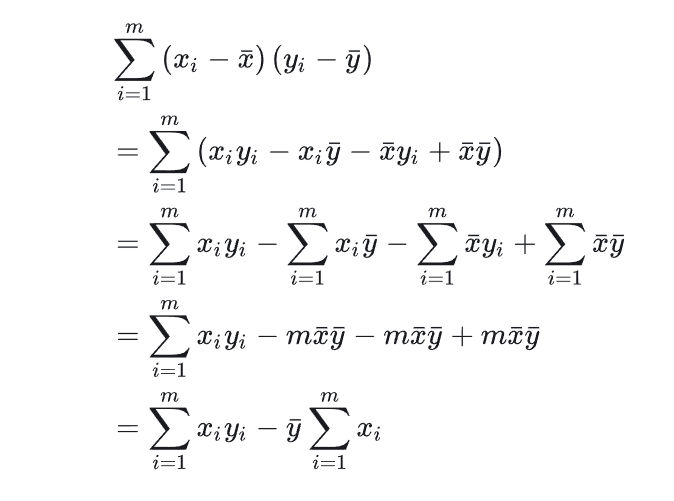
- We will have $β_{1} = \frac{C o v (X, Y)}{V a r (X)}$

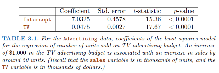
2.1.2. Assessing the Accuracy of Coefficient Estimates#

$S E (β_{1})^{2} = \frac{σ^{2}}{\sum_{i = 1}^{n} (x - \bar{x})^{2}}$
$S E (β_{0})^{2} = σ^{2} [\frac{1}{n} + \frac{{\bar{x}}^{2}}{\sum_{i = 1}^{n} (x_{i} - \bar{x})^{2}}]$
- Where $σ^{2} = V a r (e)$
These two standard errors can be used to compute confidence interval, for example, for 95% confidence interval, it has the form [ $β_{1} - 2 * S E (β_{1})$ , $β_{1} + 2 * S E (β_{1})$ ]

2.1.3. Hypothesis Testing#

Standard errors can be used to perform hypothesis tests on coefficients.
To test the null hypothesis, we compute a t-statistic, given by
$t = \frac{β_{1} - 0}{S E (β_{1})}$
- This value follows a t-distribution with n-2 degrees of freedom
- $H_{0}$ assumes $β_{1} = 0$
- Since $H_{0} : β_{1} = 0$ , [ $β_{1} - 2 * S E (β_{1})$ , $β_{1} + 2 * S E (β_{1})$ ] should not contain 0

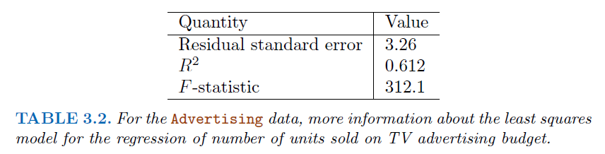
2.1.4. Assessing the Overall Accuracy of the Model#

We compute the Residual Standard Error

$R S E = \sqrt{\frac{1}{n - 2} R S S} = \sqrt{\frac{1}{n - 2} \sum_{i}^{n} (y_{i} - {\hat{y}}_{i})^{2}}$
- Where RSS is the residual sum-of-squares
We can also use R-squared (fraction of variance explained):

$R^{2} = \frac{T S S - R S S}{T S S} = 1 - \frac{R S S}{T S S}$
- Where $T S S = \sum_{i = 1}^{n} (y_{i} - \bar{y})^{2}$ , is the total sum of squares
- Also, In the simple linear regression setting, $R^{2} = r^{2}$ where $r$ is the correlation between $X$ and $Y$ :
$r = \frac{\sum_{i = 1}^{2} (x_{i} - \bar{x}) (y_{i} - \bar{y})}{\sqrt{\sum_{i = 1}^{2} (x_{i} - \bar{x})^{2}} \sqrt{\sum_{i = 1}^{2} (y_{i} - \bar{y})^{2}}}$

# Example data
x = np.array([1., 2., 3., 4., 5.]).reshape(-1, 1)
y = np.array([2., 4., 5., 8., 7.])

# Calculating means
x_mean = np.mean(x)
y_mean = np.mean(y)

# Calculating Beta_1
numerator = sum([i*j for i,j in zip(x-x_mean,y-y_mean)])
denominator = np.sum((x - x_mean)**2)
beta_1 = numerator / denominator

print("Beta_1 (slope) using OLS:", beta_1)

Beta_1 (slope) using OLS: [1.4]

2.1.5. Maximum likelihood estimation#

In the context of linear regression, MLE assumes that the residuals (differences between observed and predicted values) are normally distributed.
The method finds the parameter values that maximize the likelihood of observing the given data.

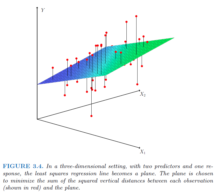
2.2. Multiple Linear Regression#

$Y = β_{0} + β_{1} X_{1} + β_{2} X_{2} + . . . + β_{p} X_{p} + e$

Correlations amongst predictors cause problems (multicollinearity):
- The variance of all coefficient tends to increase, sometimes dramatically.
- $t = \frac{β_{1} - 0}{S E (β_{1})}$ , If $S E (β_{1})$ becomes larger, will contributes to a $t$ closer to 0, which will lead to a larger p-value
- Also, it’s hard to interpret.
Claims of causality should be avoided!

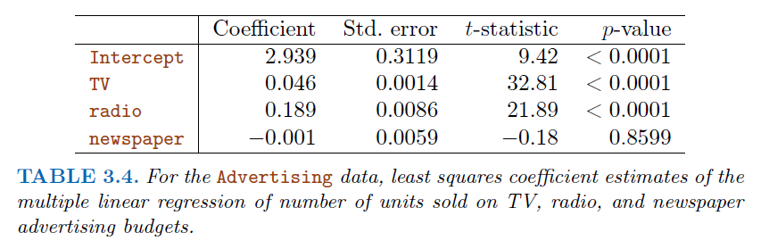
2.2.1. Important Question (Hypothesis testing)#

Is at least one of the predictors $X_{1}, X_{2}, . . ., X_{p}$ useful in predicting the response?
- For this question, we use the $F - s t a t i s t i c$
- $F = \frac{(T S S - R S S) / p}{R S S / (n - p - 1)}$ ~ $F_{p, n - p - 1}$
  - Where $n$ is the number of observations, $p$ is the number of predictors
- $H_{0} :$ None of these predictors are useful
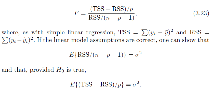
- If $H_{0}$ is false, we expect $F > 1$
Do all the predictors help to explain $Y$ , or is only a subset of the predictors useful?
- Forward Selection
  - Begin with the null model
  - Fit p simple linear regression and add the null model the variable results in the lowest RSS
  - Add to that model the variable that results in the lowest RSS amongst all two-variable models.
  - Continue until stopping rules is satisfied (e.g. p-value >0.05 for all remaining variables)
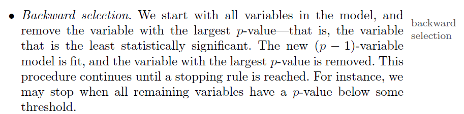
- Backward Selection
- Model Selection
  - Besides RSS, there are some other criteria for choosing an “optimal” member in stepwise searching, including Akaike information criterion (AIC), Bayesian information criterion (BIC), adjusted R-squared
How well does the model fit the data?
Given a set of predictor values, what response value should we predict, and how accurate is our prediction?

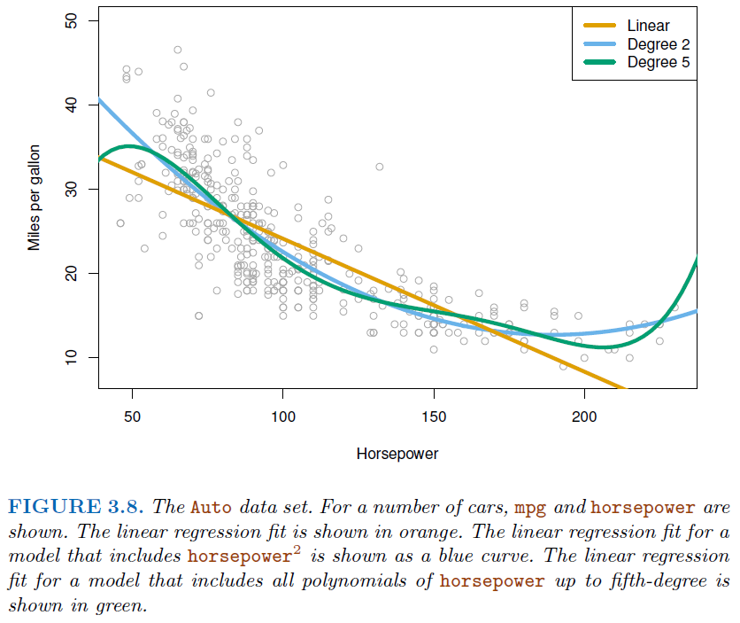
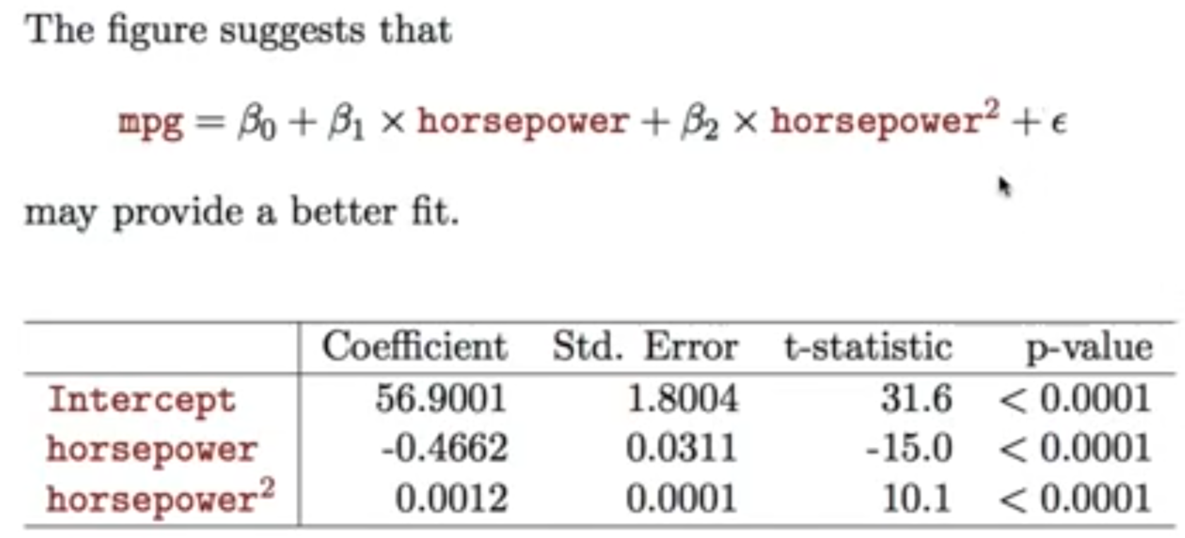
2.2.2. Polynomial regression (non-linear effects)#

2.3. Interesting Quotes by famous Statisticians#

Essentially, all models are wrong, but some are useful
- George Box
The only way to find out what will happen when a complex system is disturbed is to disturb the system, not merely to observe it passively
- Fred Mosteller and John Tukey, paraphrasing George Box

Regression

Contents

2. Regression#

2.1. Simple Linear Regression#

2.1.1. Find Best estimator of β1#

2.1.1.1. Ordinary Least Squares#

2.1.2. Assessing the Accuracy of Coefficient Estimates#

2.1.3. Hypothesis Testing#

2.1.4. Assessing the Overall Accuracy of the Model#

2.1.5. Maximum likelihood estimation#

2.2. Multiple Linear Regression#

2.2.1. Important Question (Hypothesis testing)#

2.2.2. Polynomial regression (non-linear effects)#

2.3. Interesting Quotes by famous Statisticians#

2.1.1. Find Best estimator of $β_{1}$ #