4. Sampling

• Sometimes we need to test the model performance, but we can not use the same data as training and testing. therefore we need sampling strategies.

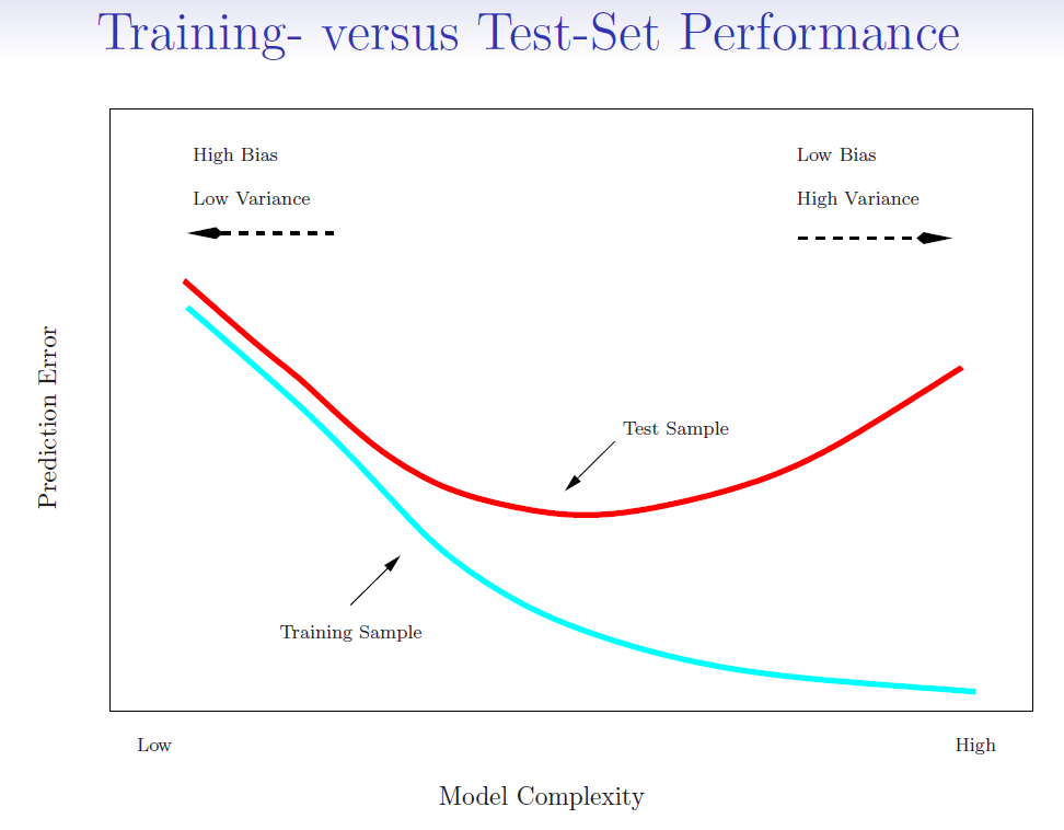
• Training error (blue line): Training error, also known as in-sample error, is the error that occurs when a model is applied to the data it was trained on.

• Testing error (red line): Testing error, or out-of-sample error, is the error that occurs when the model is applied to a new dataset that it hasn’t seen before, often a validation or test set.

4.1. Estimate Testing error

• When we use training error to estimate testing error, we often get a underestimated result. Some methods make a mathematical adjustment to the training error rate in order to estimate the test error rate.

  • \(-2ln(L)\) use the same way as RSS, in linear regression, \(-2log(L) = RSS/\sigma^2\)

4.1.1. AIC (Akaike Information Criterion)

\[ AIC=2k-2ln(L) \]

• \(k\) is the number of parameters in the model

• \(L\) is the maximum value of the likelihood function for the model

  • Normally, we assume errors are normally distributed (offsets between expectation and observation)

4.1.2. BIC (Bayesian Information Criterion)

\[ BIC=ln(n)k-2ln(L) \]

• \(n\) is the number of observations

• The other terms are as defined for AIC

• when \(n > 7\), \(BIC\) put more penalty than \(AIC\)

4.1.3. Example

• Want to compare linear vs higher-order polynomial terms in a linear regression

import numpy as np
import statsmodels.api as sm

# Generate some data
np.random.seed(0)
X = np.random.uniform(-10, 10, 100)
Y = 3 - 2*X + X**2 + np.random.normal(0, 2, 100)

# Fit models of varying complexity
results = {}
for degree in range(1, 6):
    features = np.column_stack([X**i for i in range(1, degree + 1)])
    features = sm.add_constant(features)
    model = sm.OLS(Y, features).fit()
    results[degree] = {'model': model, 'AIC': model.aic, 'BIC': model.bic}

# Find the best model according to AIC and BIC
best_by_aic = min(results, key=lambda k: results[k]['AIC'])
best_by_bic = min(results, key=lambda k: results[k]['BIC'])

print(f'Best model by AIC is of degree {best_by_aic} with AIC = {results[best_by_aic]["AIC"]}')
print(f'Best model by BIC is of degree {best_by_bic} with BIC = {results[best_by_bic]["BIC"]}')

Best model by AIC is of degree 2 with AIC = 425.7373213865948
Best model by BIC is of degree 2 with BIC = 433.55283194455905

4.2. Cross Validation

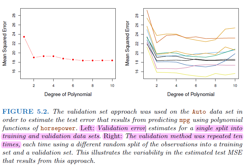
• In normal validation approach, only a subset of the observation are used to fit the model

  • The validation error may tend to overestimate the test error for the model fit on the entire data set

  • For some shrinkage method (e.g. Lasso and Ridge regression), it’s hard to find the number of predictors \(k\)

  • Cross validation provide a direct way to test error, instead of using the variance of error \(\sigma^2\)

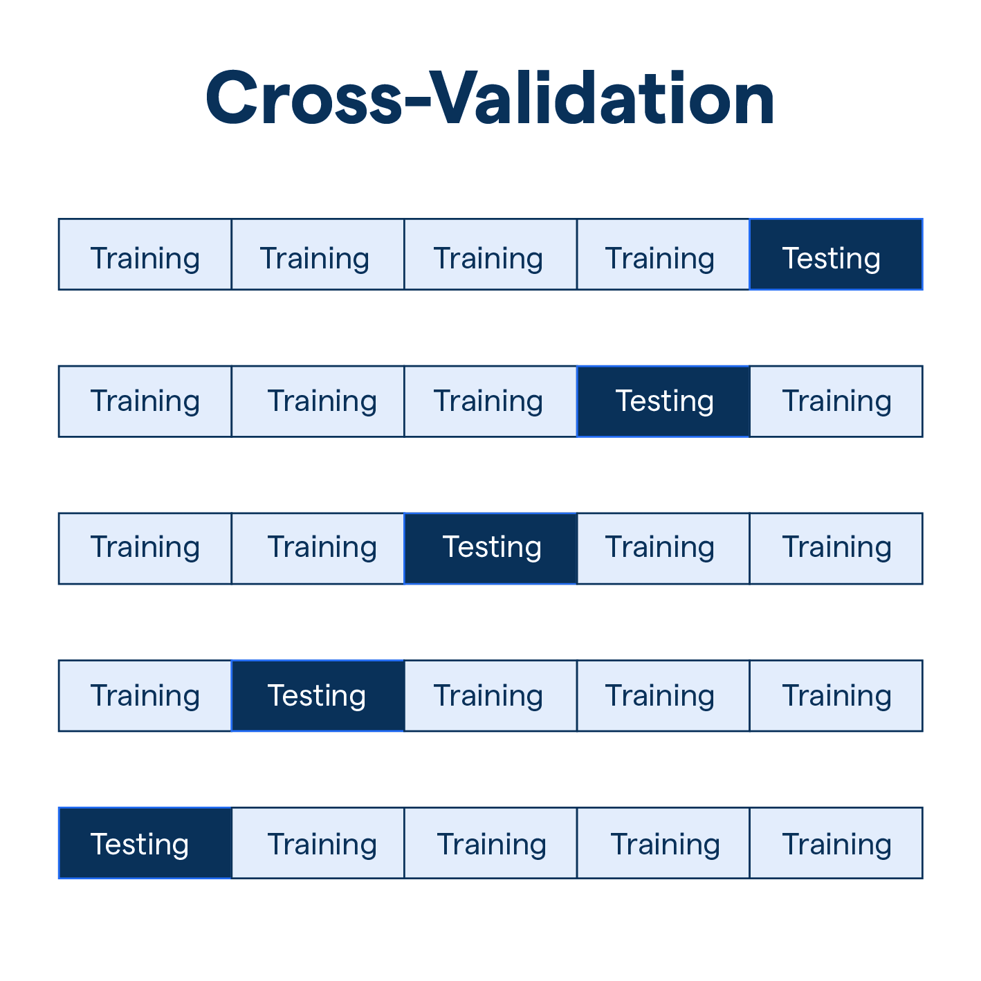
4.2.1. K-fold Cross Validation

• Let the \(K\) parts be \(C_1,C_2,...,C_K\), where \(C_k\) denotes the indices of the observations in part \(k\). There’re \(n_k\) observations in part k, where \(n_k=n/K\)

• Compute (regression)

  \[ CV_{(K)}=\sum_{k=1}^K\frac{n_k}{n}MSE_k \]

• For Classification, Compute * Where \(Err_k = \sum_{i\in C_k}I(y_i\neq \hat{y_i})/n_k\) $\( CV_{(K)}=\sum_{k=1}^K\frac{n_k}{n}Err_k \)$

• basically the weighted sum of \(MSE_k\) by number of observations in \(k\)

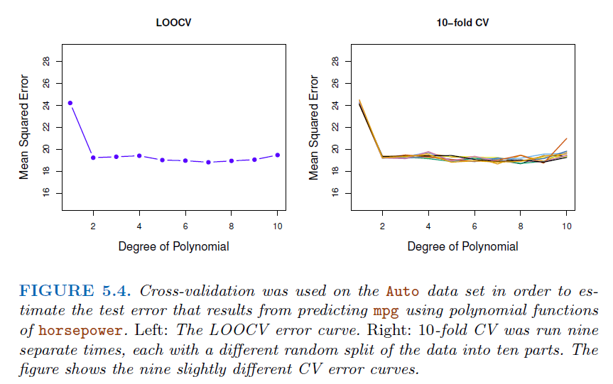
• Since each training set is only \((K-1)/K\), the estimates of prediction error will typically be biased upward.

• \(K=5\) or \(10\) provides a good compromise for bias-variance tradeoff.

4.2.2. Example using Cross Validation

4.2.3. Common mistakes in Cross Validation

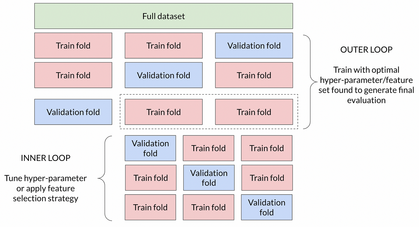
4.2.3.1. Feature selection before Cross validation

• Performing feature selection before cross-validation can lead to data leakage and overfitting, as you’re peeking at the entire dataset to select features based on their correlation with the target variable.

• This can result in overly optimistic performance estimates.

4.2.3.2. Example

• We randomly generate 50 predictors with different mean and variance normal distribution, and random label Y

• We select 5 predictors having the largest correlation with the radom label

• Then we put this 5 predictors into logistic regression to get CV Score

• Theoretically, we will get CV score around 50% since the independent simulation, but result gives us much higher score

from sklearn.model_selection import cross_val_score
from sklearn.linear_model import LogisticRegression
from scipy.stats import pearsonr

# Set random seed for reproducibility
np.random.seed(5)

# Generate X with 50 random arrays following normal distribution with different mean and variance
X = np.random.normal(loc=np.random.uniform(-10, 10, size=50), scale=np.random.uniform(1, 5, size=50), size=(100, 50))

# Generate y as random labels from uniform distribution
y = np.random.randint(2, size=100)

# Step 2: Select the 5 features most correlated with the outcome
## This step is wrong since model have seen 
## all labels to get most correlated predictors
correlations = np.array([pearsonr(X[:, i], y)[0] for i in range(X.shape[1])])
top_five_indices = np.argsort(np.abs(correlations))[-5:]

# Step 3: Perform cross-validation using only the selected features
selected_X = X[:, top_five_indices]
model = LogisticRegression()

# Use cross-validation to estimate the test error
cv_scores = cross_val_score(model, selected_X, y, cv=5)

# The mean cross-validated score can be misleadingly high due to feature selection bias
mean_cv_score = np.mean(cv_scores)
print("Cross-validation scores:", cv_scores)
print(f'Mean CV score: {mean_cv_score}')

Cross-validation scores: [0.55 0.7  0.45 0.75 0.75]
Mean CV score: 0.64

4.3. Bootstrap

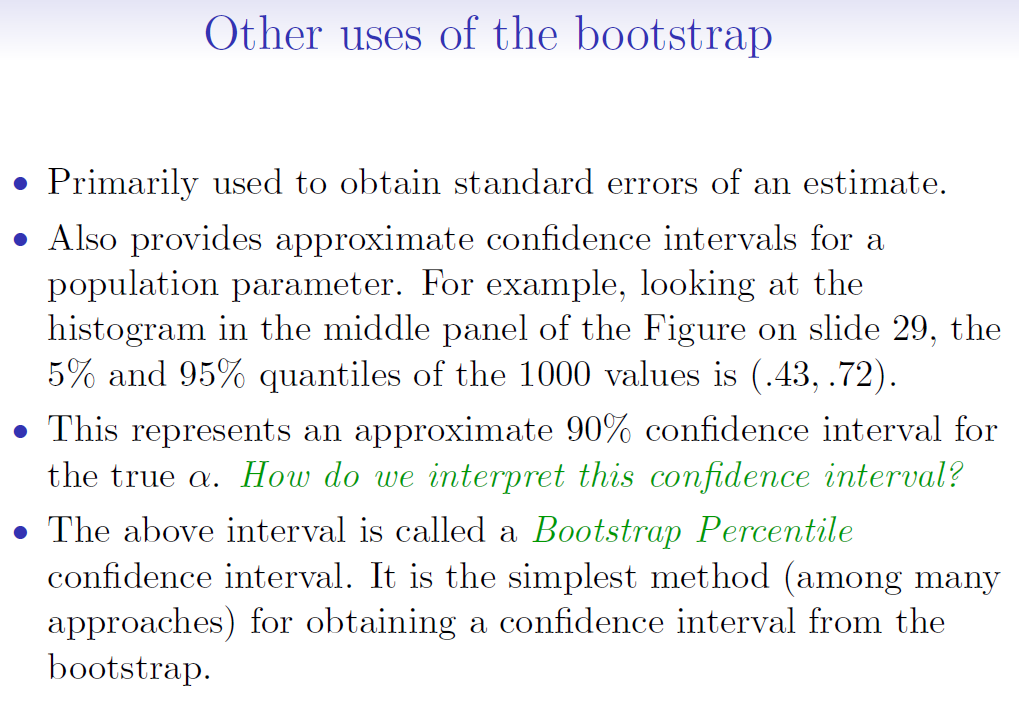
• The bootstrap is a flexible and powerful statistical tool that can be used to quantify the uncertainty associated with a given estimator or statistical learning method.

  • For example, it provides the estimate of standard error of a coefficient, or a confidence interval for that coefficient.

4.3.1. Example for Bootstrap

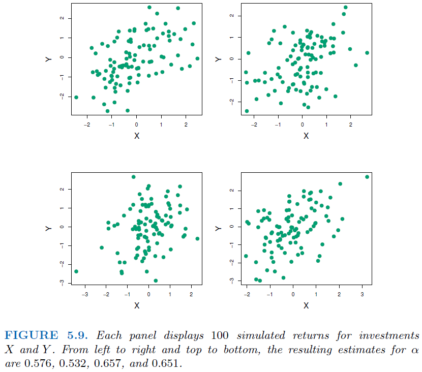
• We want to invest our money in two financial assets that yield returns of X and Y

• We will invest a fraction \(\alpha\) of our money in \(X\), and \(1-\alpha\) in Y

• We wish to choose \(\alpha\) to minimize the total risk, or variance (\(Var(\alpha X+(1-\alpha)Y)\)), of our investment. $\( Var(\alpha X+(1-\alpha)Y) = \alpha ^2Var(X) + (1-\alpha)^2 Var(Y) + 2\alpha(1-\alpha) CoV(XY) \)\( \)\( \frac{\partial f}{\partial \alpha} = 2\alpha Var(x) - 2(1-\alpha) Var(Y) + 2(1-\alpha) CoV(XY) - 2\alpha(XY) \)$

• Let \(\frac{\partial f}{\partial \alpha} = 0\), we get $\( \alpha = \frac{Var(Y)-Cov(XY)}{Var(X)+Var(Y)-2CoV(XY)} \)$

• We can estimate \(Var(X), Var(Y)\) and \(CoV(XY)\) using sampling / simulation

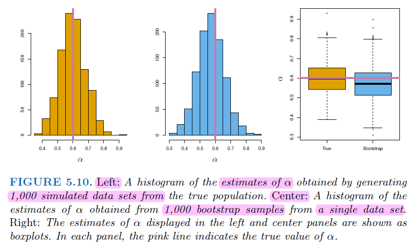
4.3.2. Why we need Bootstrap

1. In real word analysis, we cannot generate new samples from the original population.

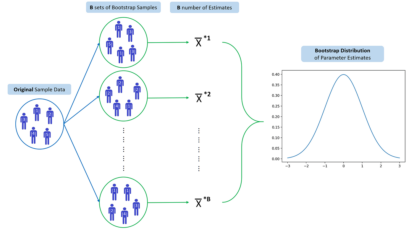
   • Bootstrap allows us to mimic the process of obtaining new data sets. So we can estimate the variability of our estimate without generating additional samples

   • Each bootstrap datasets is created by sampling with replacement, and is the same size as the original dataset.

   • There is about a two-thirds overlap in a bootstrap sample with the original data

   

2. Bootstrap requires data being independent to each other, some data like time series are not applicable for Bootstrap

   • For time series, we can divide data by blocks, then use block to do bootstrap