Autograd

12. Autograd#

Reference
Learning Material for Differential
Learning Material for Linear Algbra
Learning Material for Linear Algbra (Video)

Frameworks like torch are so popular because of what you can do with them: deep learning, machine learning, optimization, large-scale scientific computation in general. * Most of these application areas involve minimizing some loss function. * This, in turn, entails computing function derivatives.

12.1. Why compute derivatives?#

The training, or learning, process, is based on comparing the algorithm’s predictions with the ground truth, a comparison that leads to a number capturing how good or bad the current predictions are. To provide this number is the job of the loss function.

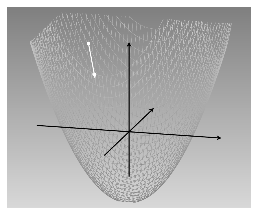
This is a quadratic function of two variables: f(x₁,x₂) = 0.2x₁² + 0..2x₂² − 5. * It has its minimum at (0,0), and this is the point we’d like to be at. * Take the x₁ direction. The derivative of the function with respect to x₁ indicates how its value varies as x₁ varies. * We can compute the partial derivative of x₁, which is $\frac{\partial f}{\partial x_1}=0.4x_1$. * This tells us that as x₁ increases, loss increases, and how fast. * The same holds for the x₂. * We want to take the direction opposite to where the derivative points.

Overall, this yields a descent direction of [−0.4x₁,−0.4x₂]

Descriptively, this strategy is called steepest descent. Commonly referred to as gradient descent, it is the most basic optimization algorithm in deep learning.

12.2. Automatic differentiation example#

Now that we know why we need derivatives, let’s see how automatic differentiation (AD) would compute f(x₁,x₂) = 0.2x₁² + 0..2x₂² − 5

This fig is how our above function could be represented in a computational graph.

x1 and x2 are input nodes, corresponding to function parameters x₁ and x₂, x7 is the function’s output

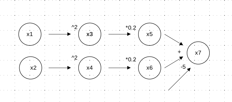In reverse-mode AD, the flavor of automatic differentiation implemented by torch

Calculate the function’s output value (x7).

This corresponds to a forward pass through the graph.

Calculate the gradient of the output with respect to both inputs, x₁ and x₂

This is a backward pass
At x7, we calculate partial derivatives with respect to x5 and x6.
From x5, we move to the left to see how it depends on x3.
From x3, we take the final step to x.
This process applied the chain rule in derivatives, we call this process back propagation

12.3. Automatic differentiation with `torch` autograd#

In torch, the AD engine is usually referred to as autograd, and that is the way you’ll see it denoted in most of the rest of this book.

To construct the above computational graph with torch, we create “source” tensors x1 and x2.

However, if we just proceed “as usual”, creating the tensors the way we’ve been doing so far, torch will not prepare for AD. Instead, we need to pass in requires_grad = TRUE when instantiating those tensors:

(By the way, the value 2 for both tensors was chosen completely arbitrarily.)

library(torch)

x1 <- torch_tensor(2, requires_grad = TRUE)
x2 <- torch_tensor(2, requires_grad = TRUE)

Now, to create “invisible” nodes x3 to x6 , we square and multiply accordingly. Then x7 stores the final result.

x3 <- x1$square()
x5 <- x3 * 0.2

x4 <- x2$square()
x6 <- x4 * 0.2

x7 <- x5 + x6 - 5
x7

## torch_tensor
## -3.4000
## [ CPUFloatType{1} ][ grad_fn = <SubBackward1> ]

Note that we have to add requires_grad = TRUE when creating the “source” tensors only. All dependent nodes in the graph inherit this property. For example

x7$requires_grad

## [1] TRUE

Now, all prerequisites are fulfilled to see automatic differentiation at work.

All we need to do to determine how x7 depends on x1 and x2 is call backward():

x7$backward()

Due to this call, the $grad fields have been populated in x1 and x2

x1$grad

## torch_tensor
##  0.8000
## [ CPUFloatType{1} ]

x2$grad

## torch_tensor
##  0.8000
## [ CPUFloatType{1} ]

These are the partial derivatives of x7 with respect to x1 and x2, respectively.

Our partial derivative is [−0.4x₁,−0.4x₂]

Conforming to it, both amount to 0.8, that is, 0.4 times the tensor values 2 and 2.

12.4. Minimize loss function with `autograd`#

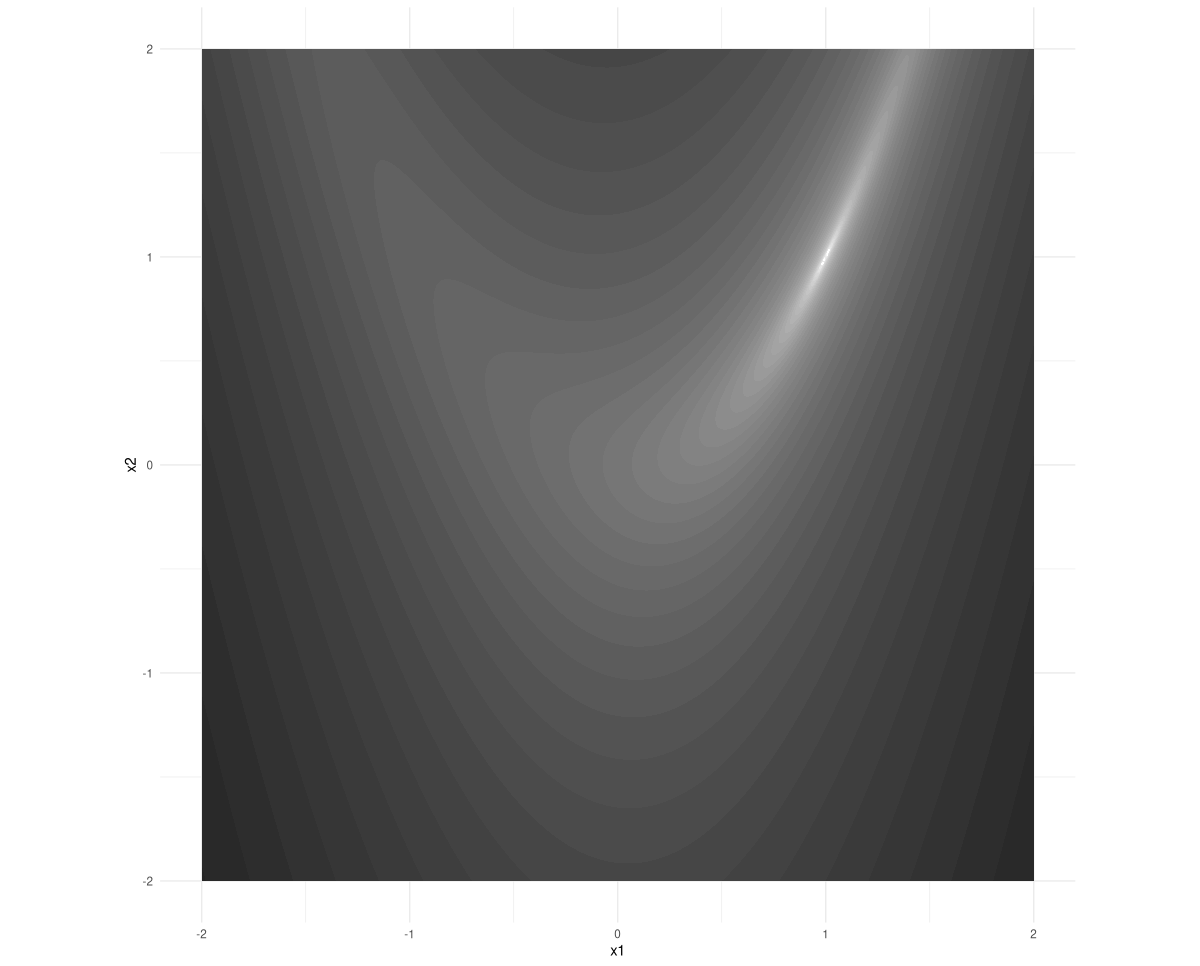
Assume we want to find x₁ and x₂ that achieve the minimum value of f when f = (1−x₁)² + 5 * (x₂−x₁²)²

Here is the function definition.

a <- 1
b <- 5

rosenbrock <- function(x) {
  x1 <- x[1]
  x2 <- x[2]
  (a - x1)^2 + b * (x2 - x1^2)^2
}

12.4.1. Minimization from scratch#

In a nutshell, the optimization procedure then looks somewhat like this:

# attention: this is not the correct procedure yet!

for (i in 1:num_iterations) {

  # call function, passing in current parameter value
  value <- rosenbrock(x)

  # compute gradient of value w.r.t. parameter
  value$backward()

  # manually update parameter, subtracting a fraction
  # of the gradient
  # this is not quite correct yet!
  x$sub_(lr * x$grad)
}

lr, for learning rate, is the fraction of the gradient to subtract on every step
num_iterations is the number of steps to take.
x is the parameter to optimize, that is, it is the function input that hopefully, at the end of the process, will yield the minimum possible function value.
- And that, in turn, means we need to create it with requires_grad = TRUE:
- x <- torch_tensor(c(-1, 1), requires_grad = TRUE)
- The starting point, (-1,1), here has been chosen arbitrarily.
torch will record all operations performed on that tensor, meaning that whenever we call backward(), it will compute all required derivatives.
- However, when we subtract a fraction of the gradient, this is not something we want a derivative to be calculated for!
- We need to tell torch not to record this action, and that we can do by wrapping it in with_no_grad().
- By default, torch accumulates the gradients stored in grad fields. We need to zero them out for every new calculation, using grad$zero_().
- Here is the sample code
```
with_no_grad({
  x$sub_(lr * x$grad)
  x$grad$zero_()
})
```

num_iterations <- 1000

lr <- 0.01

x <- torch_tensor(c(-1, 1), requires_grad = TRUE)

for (i in 1:num_iterations) {
  if (i %% 100 == 0) cat("Iteration: ", i, "\n")

  value <- rosenbrock(x)
  if (i %% 100 == 0) {
    cat("Value is: ", as.numeric(value), "\n")
  }

  value$backward()
  if (i %% 100 == 0) {
    cat("Gradient is: ", as.matrix(x$grad), "\n")
  }

  with_no_grad({
    x$sub_(lr * x$grad)
    x$grad$zero_()
  })
}

## Iteration:  100 
## Value is:  0.3502924 
## Gradient is:  -0.667685 -0.5771312 
## Iteration:  200 
## Value is:  0.07398106 
## Gradient is:  -0.1603189 -0.2532476 
## Iteration:  300 
## Value is:  0.02483024 
## Gradient is:  -0.07679074 -0.1373911 
## Iteration:  400 
## Value is:  0.009619333 
## Gradient is:  -0.04347242 -0.08254051 
## Iteration:  500 
## Value is:  0.003990697 
## Gradient is:  -0.02652063 -0.05206227 
## Iteration:  600 
## Value is:  0.001719962 
## Gradient is:  -0.01683905 -0.03373682 
## Iteration:  700 
## Value is:  0.0007584976 
## Gradient is:  -0.01095017 -0.02221584 
## Iteration:  800 
## Value is:  0.0003393509 
## Gradient is:  -0.007221781 -0.01477957 
## Iteration:  900 
## Value is:  0.0001532408 
## Gradient is:  -0.004811743 -0.009894371 
## Iteration:  1000 
## Value is:  6.962555e-05 
## Gradient is:  -0.003222887 -0.006653666

After thousand iterations, we have reached a function value lower than 0.0001. What is the corresponding (x1,x2) position?

## torch_tensor
##  0.9918
##  0.9830
## [ CPUFloatType{2} ][ requires_grad = TRUE ]

12.5. Lab#

How to use autograd in torch to solve β₀ and β₁ for y = 1 + x + e, where e ~ normal(0,0.25)

Starter code as below:

set.seed(1)
b0 <- 1; b1 <- 1; n <- 200
x <- runif(n,0,2)
y <- b0 + b1*x + rnorm(n, sd=0.25)